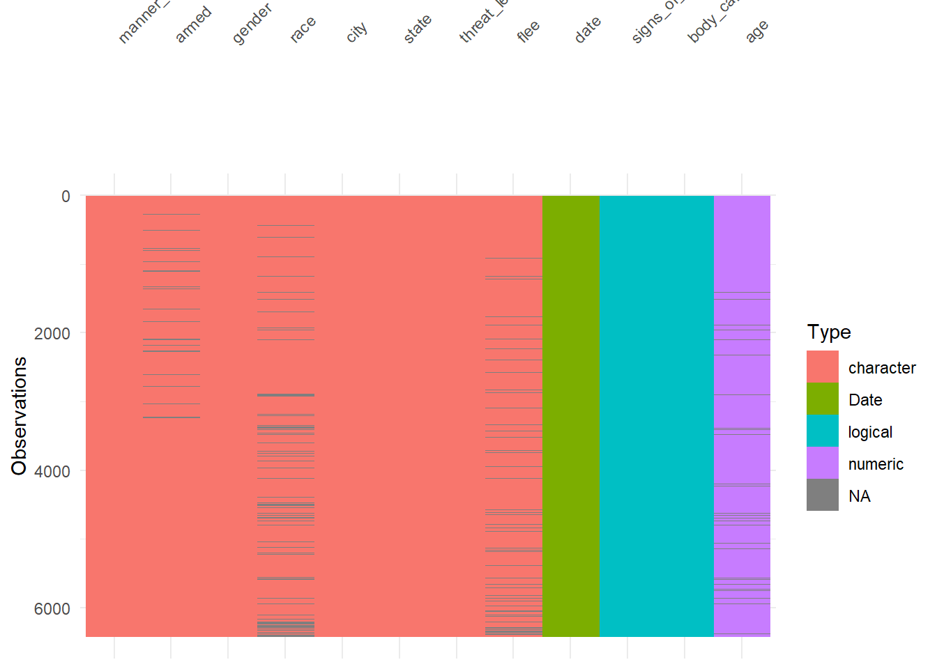
Rows: 6,421
Columns: 12
$ date <date> 2015-01-02, 2015-01-02, 2015-01-03, 2015-01-0…
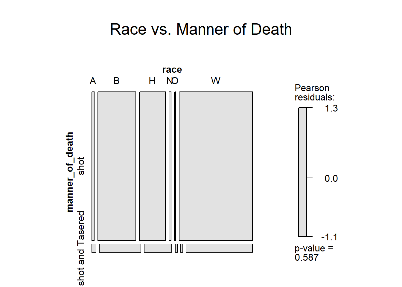
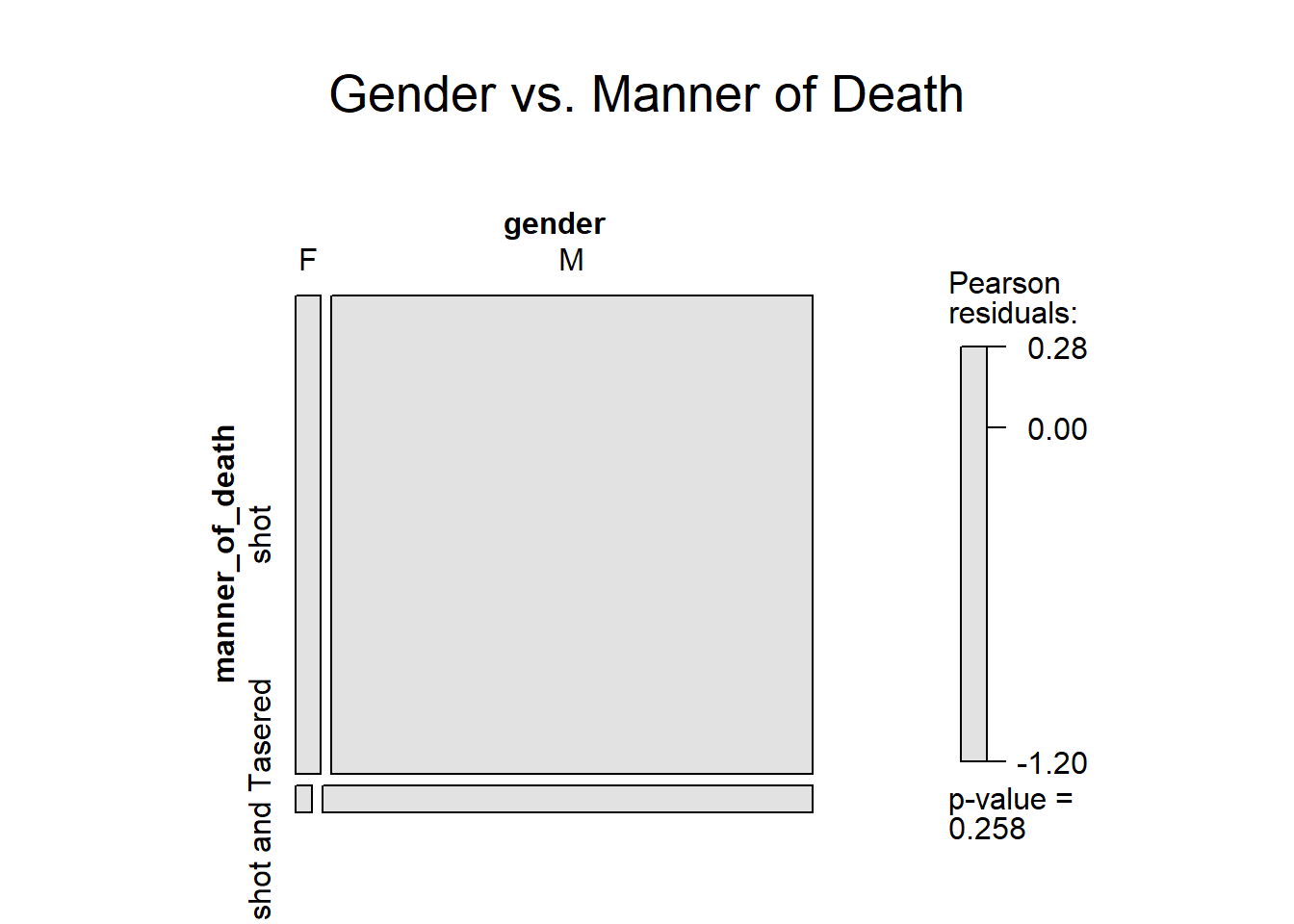
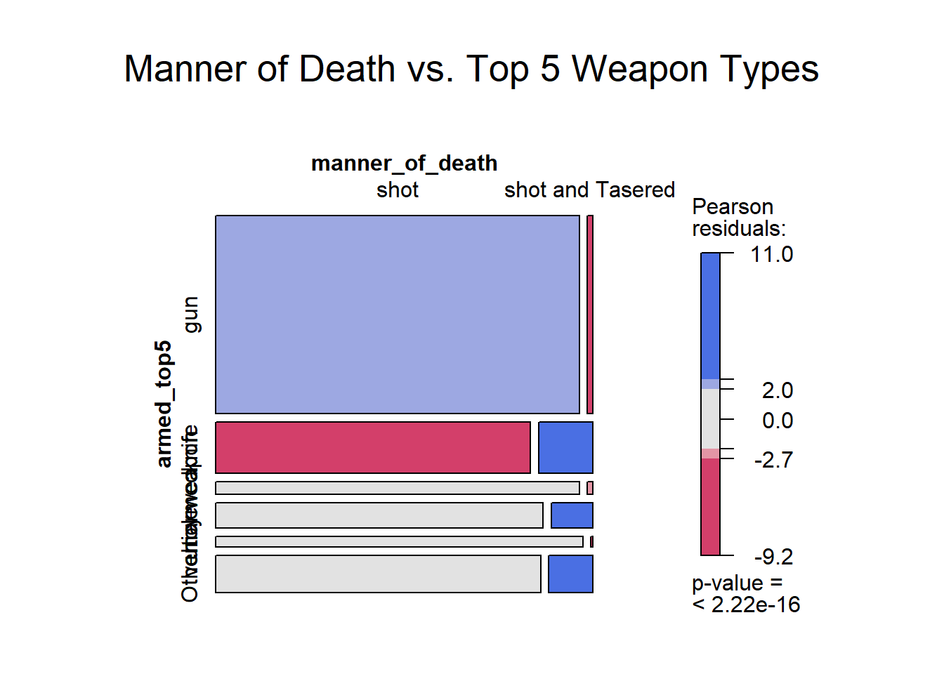
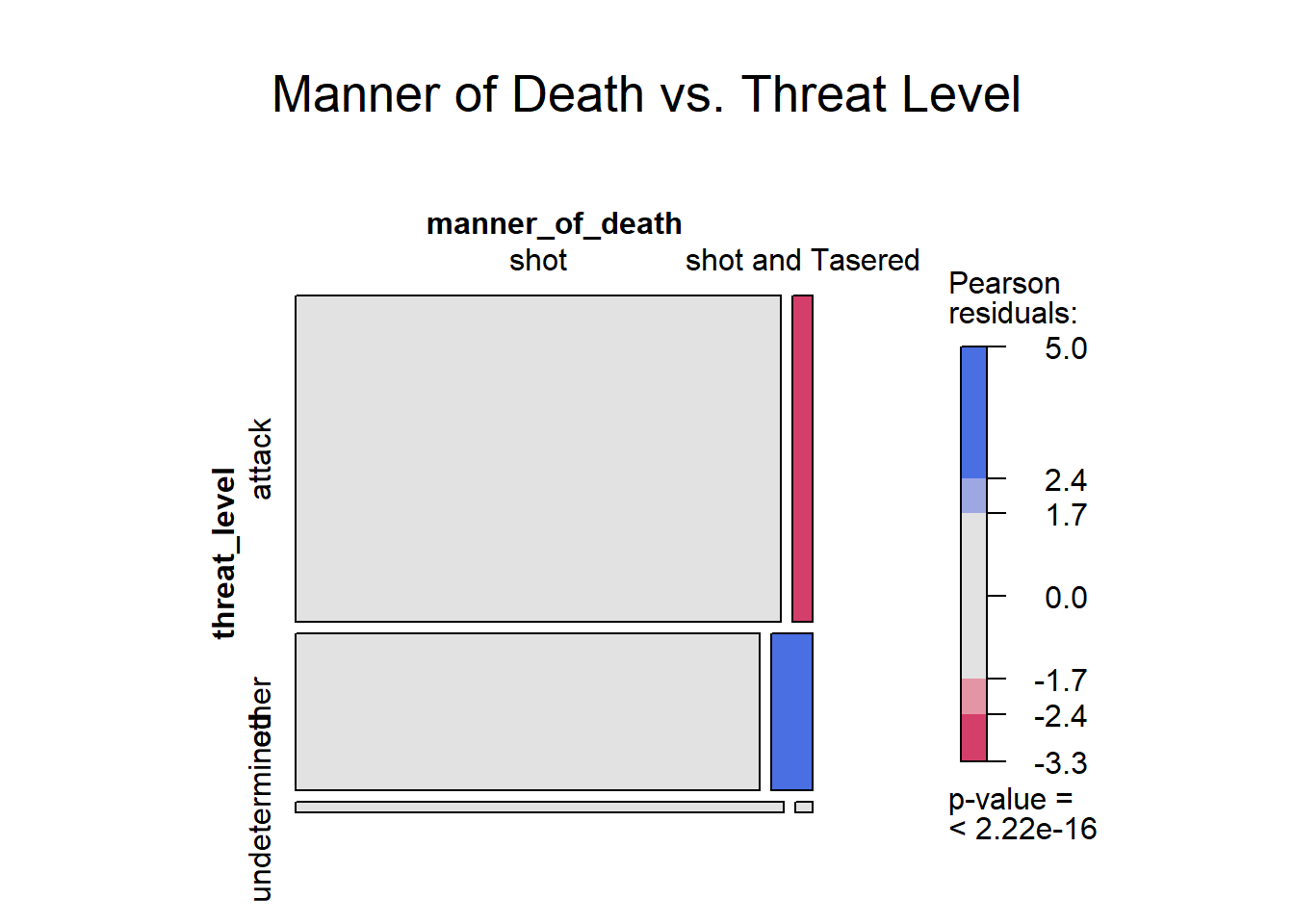
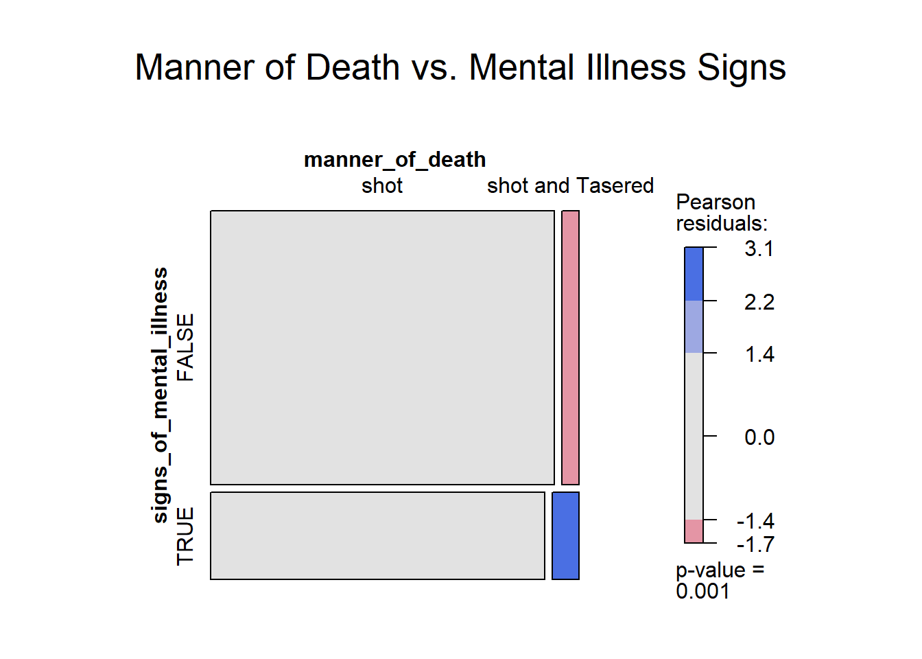
$ manner_of_death <chr> "shot", "shot", "shot and Tasered", "shot", "s…
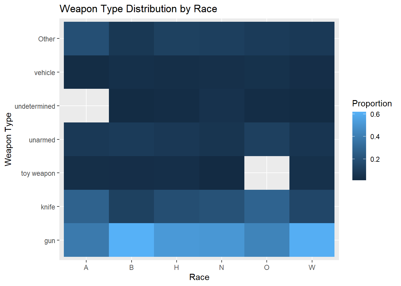
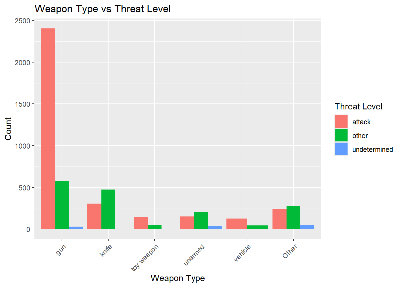
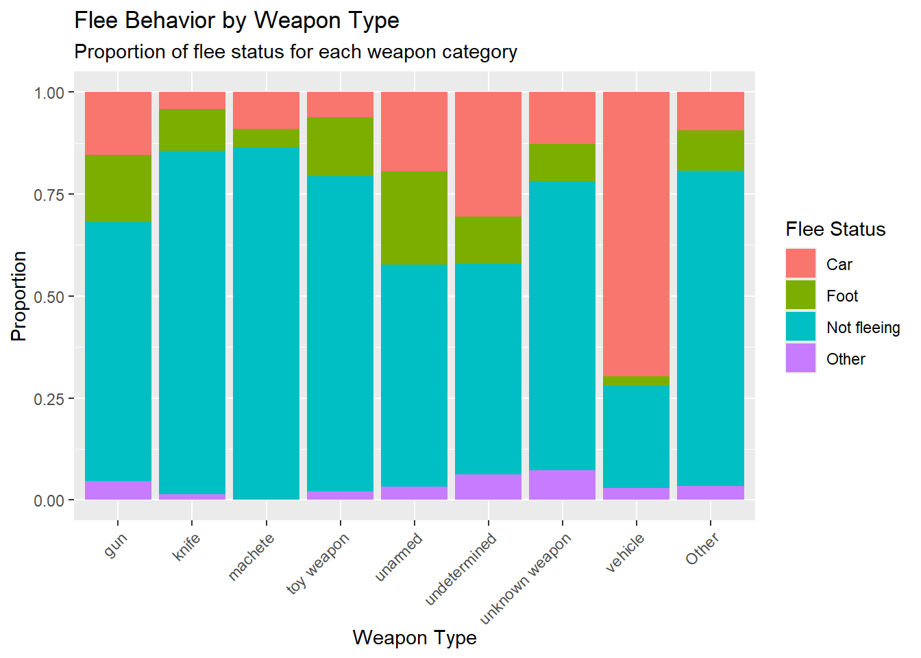
$ armed <chr> "gun", "gun", "unarmed", "toy weapon", "nail g…
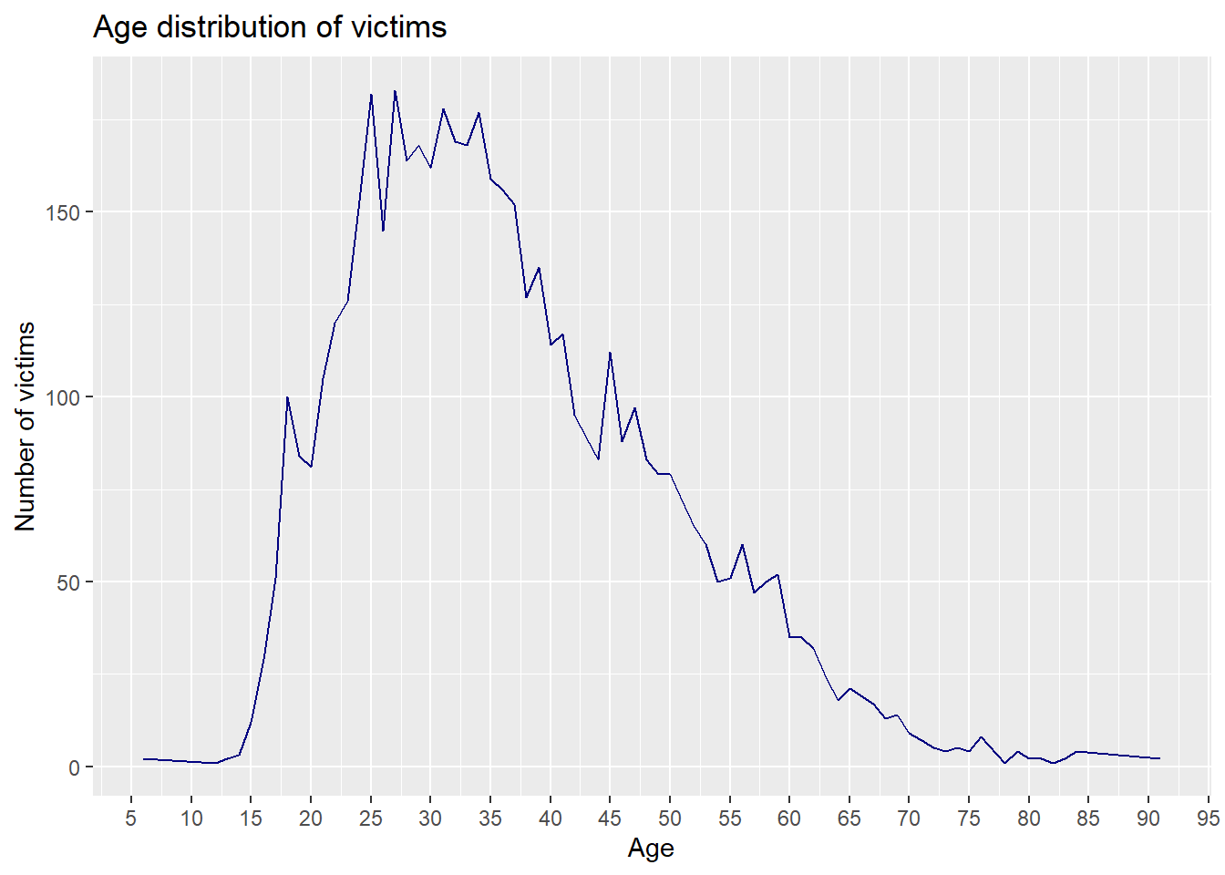
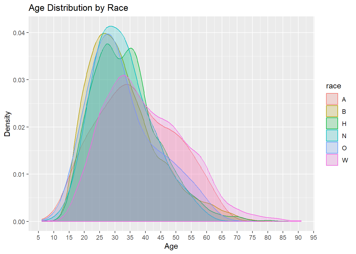
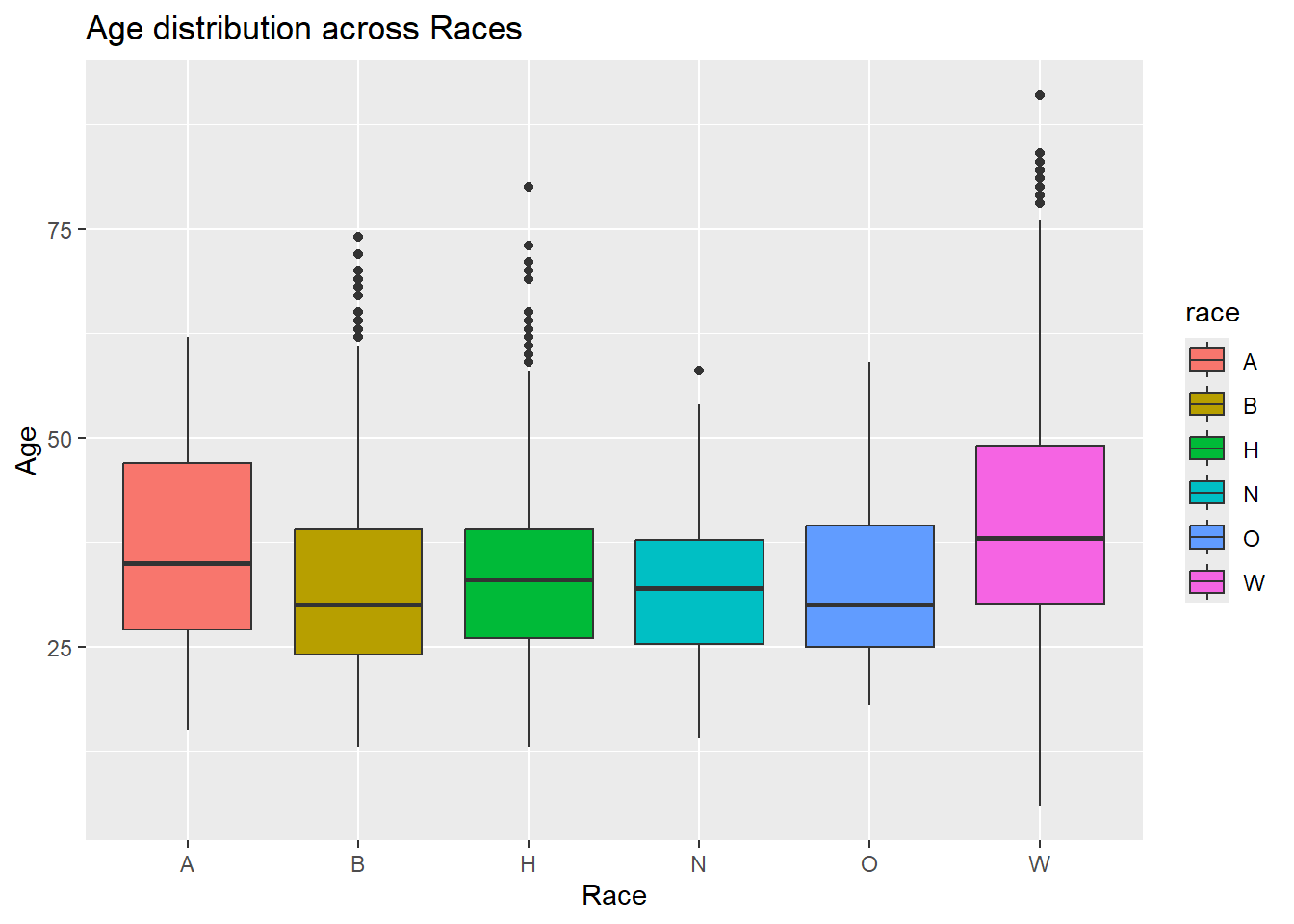
$ age <dbl> 53, 47, 23, 32, 39, 18, 22, 35, 34, 47, 25, 31…
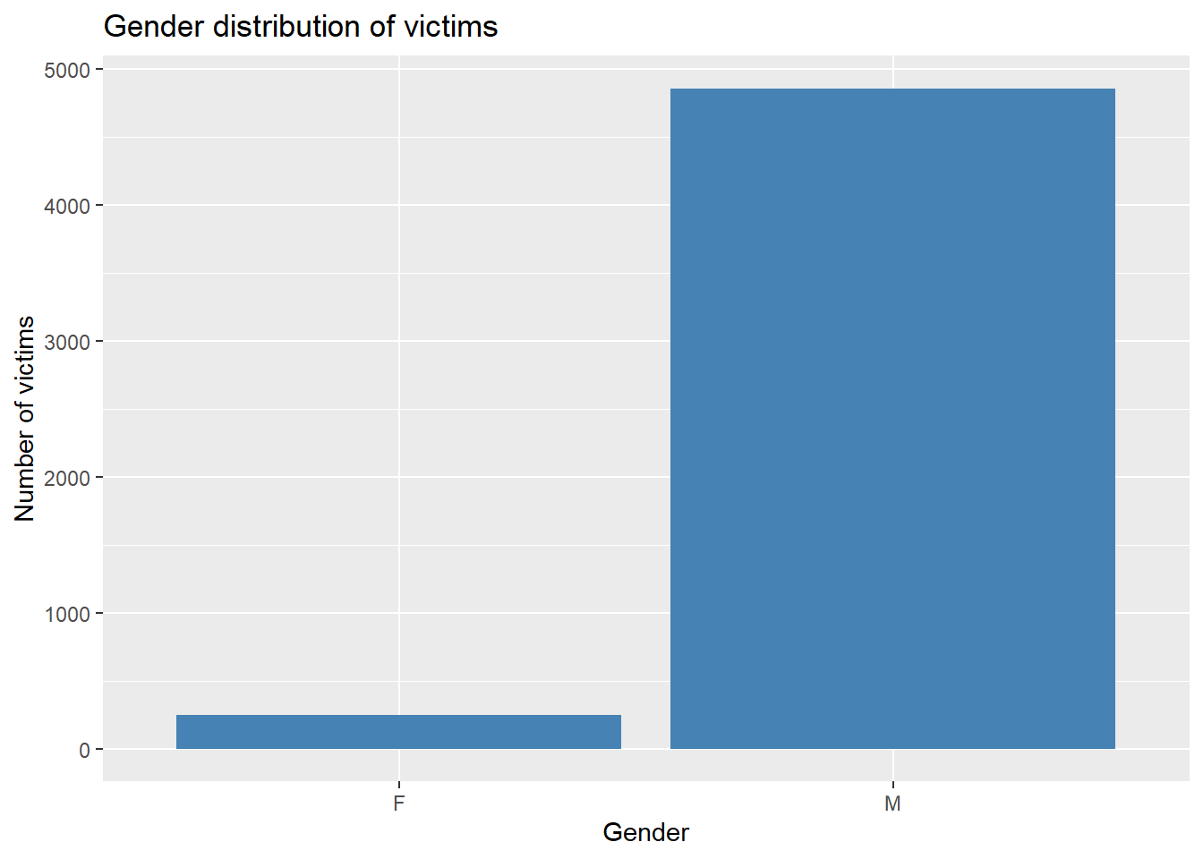
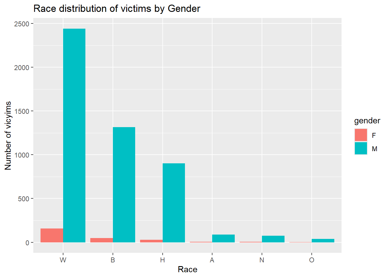
$ gender <chr> "M", "M", "M", "M", "M", "M", "M", "M", "F", "…
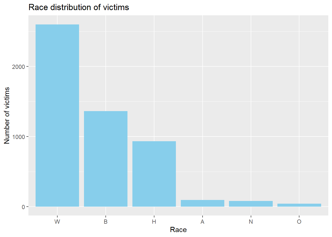
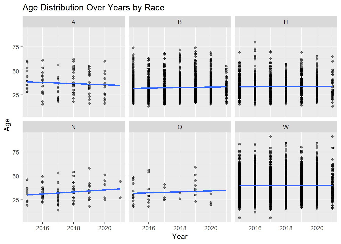
$ race <chr> "A", "W", "H", "W", "H", "W", "H", "W", "W", "…
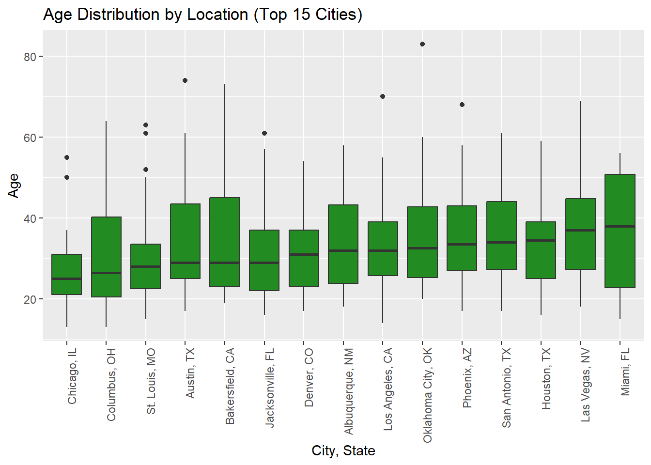
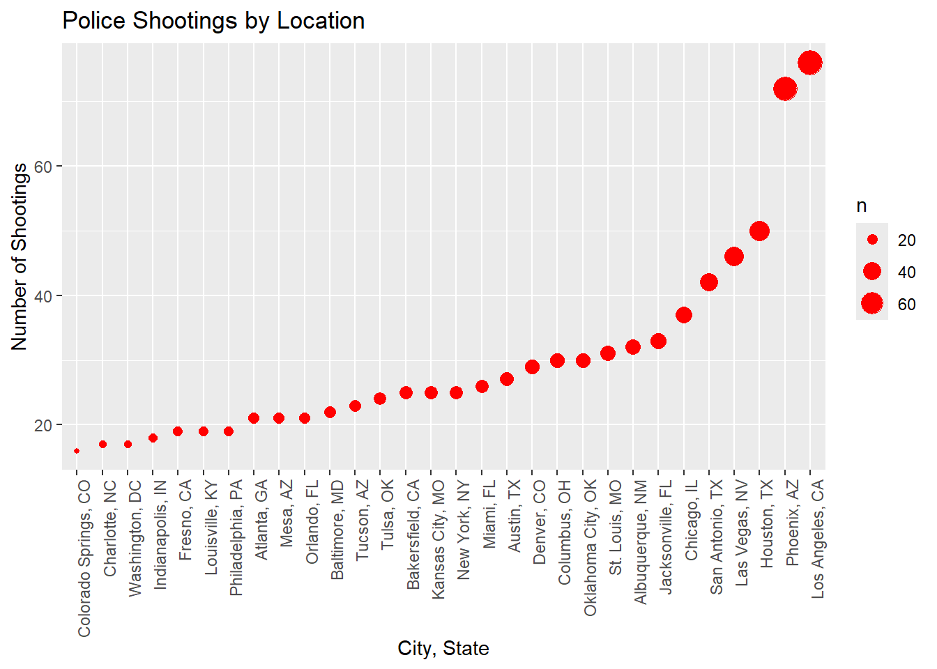
$ city <chr> "Shelton", "Aloha", "Wichita", "San Francisco"…
$ state <chr> "WA", "OR", "KS", "CA", "CO", "OK", "AZ", "KS"…
$ signs_of_mental_illness <lgl> TRUE, FALSE, FALSE, TRUE, FALSE, FALSE, FALSE,…
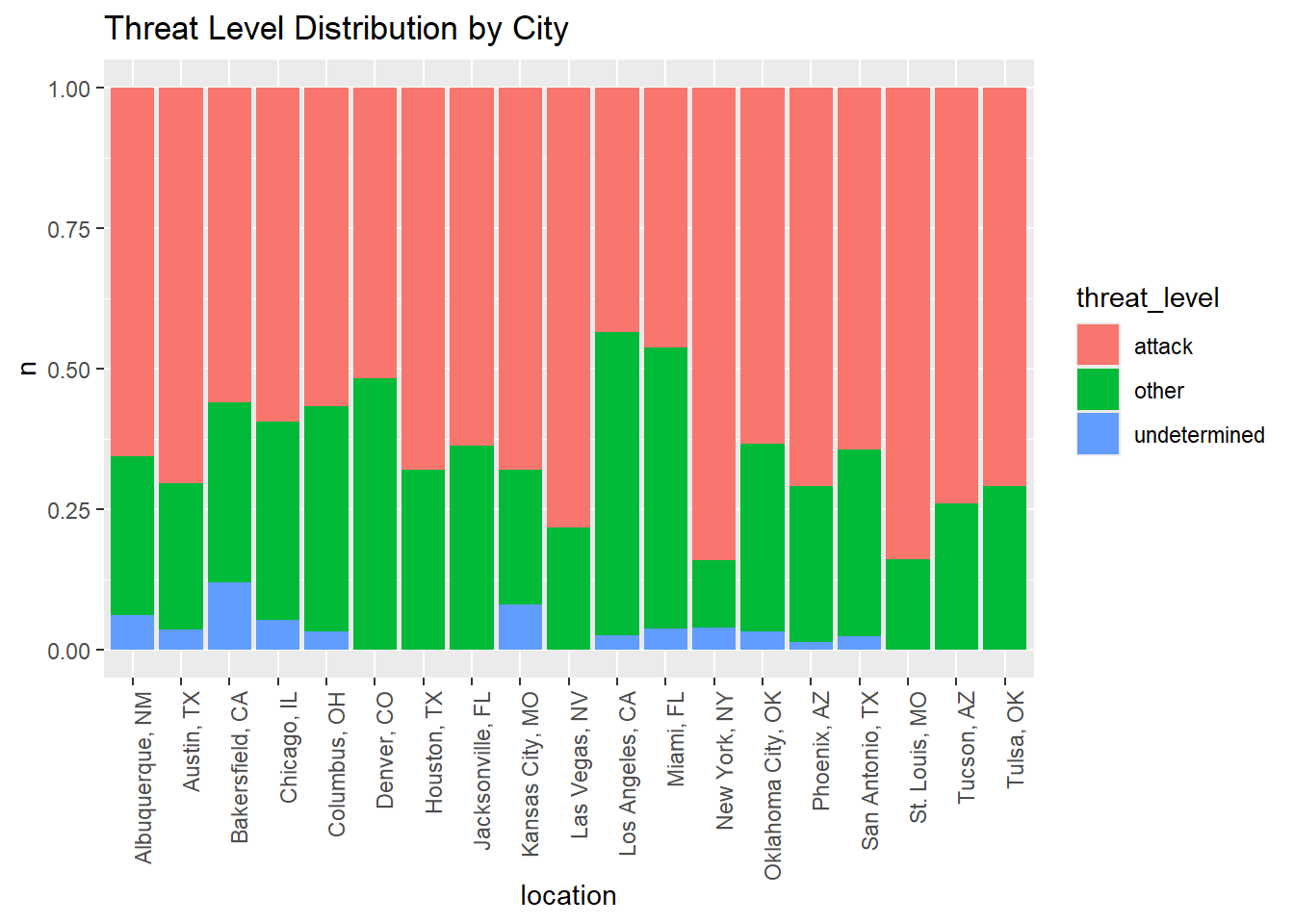
$ threat_level <chr> "attack", "attack", "other", "attack", "attack…
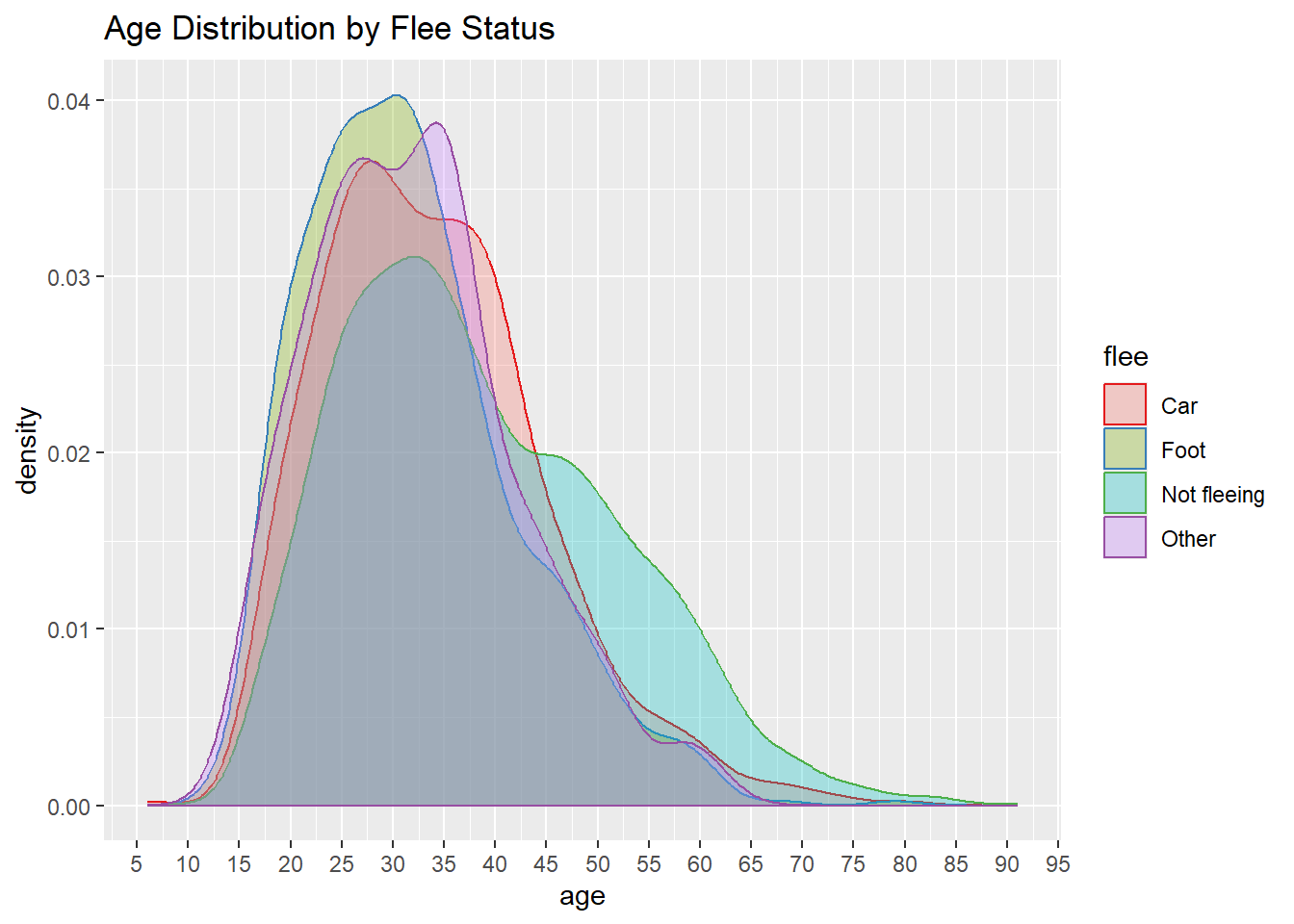
$ flee <chr> "Not fleeing", "Not fleeing", "Not fleeing", "…
$ body_camera <lgl> FALSE, FALSE, FALSE, FALSE, FALSE, FALSE, FALS…