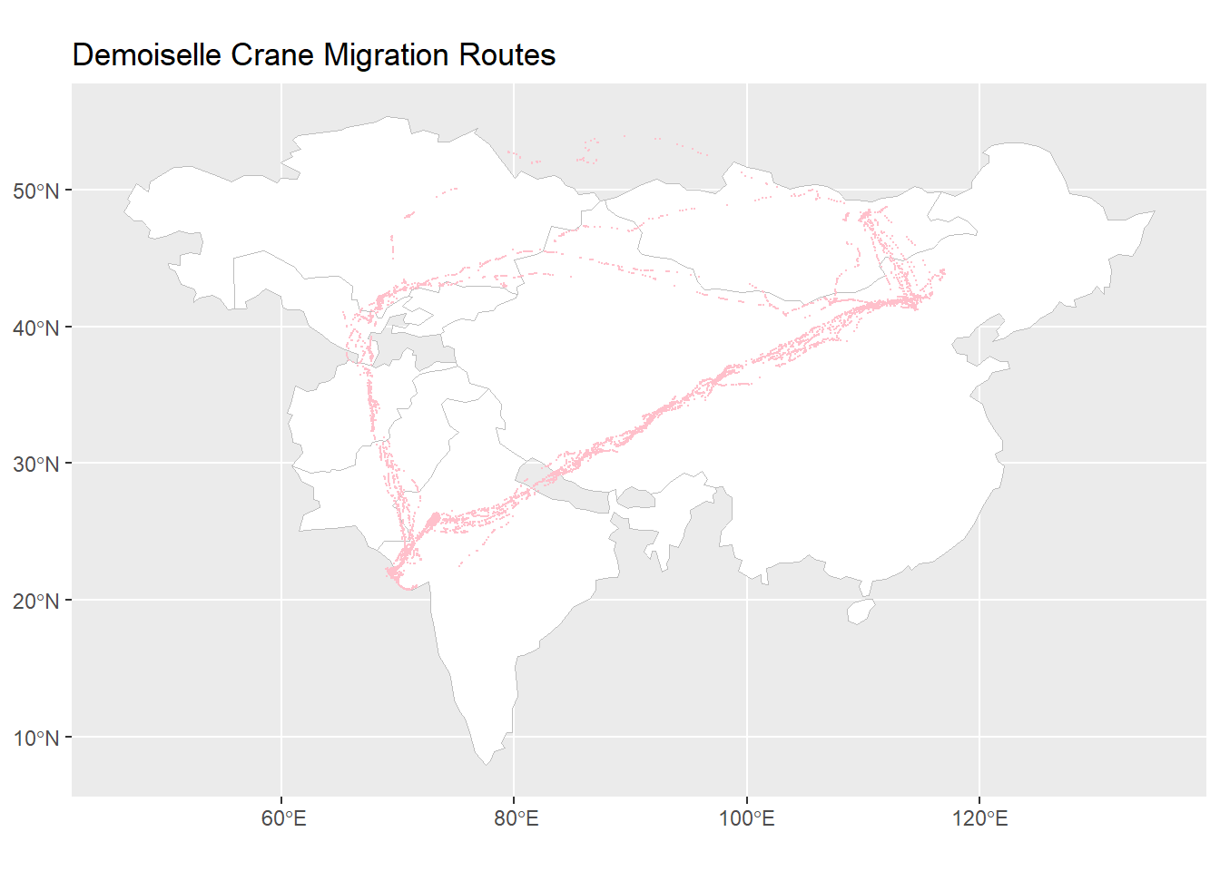
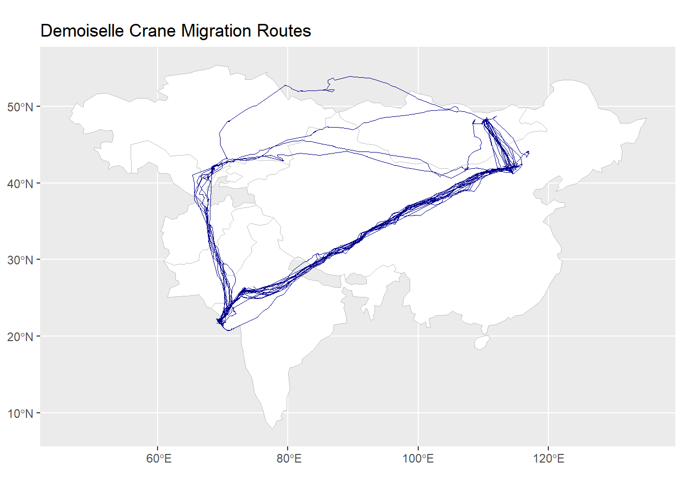
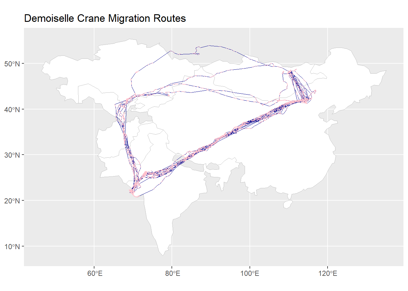
Mapping out the migration route of the Demoiselle Crane
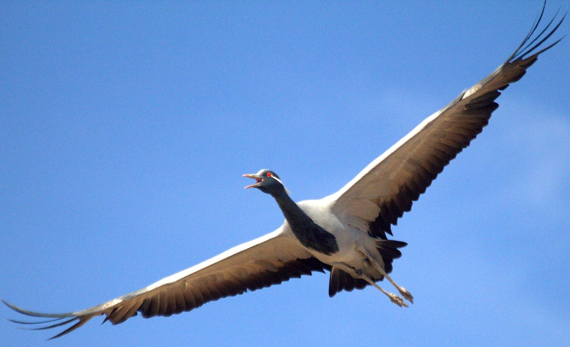
The Demoiselle Crane (aka Anthropoides virgo) has the most remarkable migration pattern. Every year, it travels around thousands of kilometers between its breeding grounds in Central Eurasia (from Ukraine and Mongolia to China) and its wintering areas in India and Africa. It’s known for its elegance and graceful movements among the crane species. (Fun fact: Its also the smallest among the crane species!)
Migration patterns
During migration, the birds fly in large flocks and often cross the Himalayas. Crossing the Himalayas is an insane thing to do - that too without oxygen tanks, in freezing -20-degree Celsius winds! They use thermal air currents and favorable winds to conserve their energy. They fly in V shaped formations for better aerodynamics. In spring they take a longer route around the cold Tibetan Plateau which saves them time and in Autumn they choose a shorter and higher route which is directly above it which saves them a lot of energy. They migrate in families with adults guiding their young ones, which shows the strong social bond among them which is crucial for such long journeys.
Why do they come to India?
They mainly come to India to avoid the harsh winters of central Asia and Mongolia; India gives them a warm welcome (literally) during the cold northern winters. They easily find leftover grains and seeds from post-harvest farmlands. Open fields, wetlands, shallow are safe and comfortable habitats for them for resting and feeding. Localities in Khichan, Rajasthan feed these birds daily which makes them feel safe. Over generations, cranes have learned and passed down this traditional migratory route and hence they return to the same areas every year. The Bishnoi communities in Rajasthan and Gujarat respect and protect these cranes reflecting India’s tradition of coexistence with nature. Their arrival marks a time for celebration in some local communities. As spring approaches, they begin their return journey towards the north to breed again in the vast Eurasian steppes.
Setup
library(rnaturalearth)library(rnaturalearthdata)
Attaching package: 'rnaturalearthdata'
The following object is masked from 'package:rnaturalearth':

    countries110
# Run this in your console first# devtools::install_github("ropensci/rnaturalearthhires")library(rnaturalearthhires)# Plotting Mapslibrary(tidyverse) # Maps using ggplot() + geom_sf()
── Conflicts ────────────────────────────────────────── tidyverse_conflicts() ──
✖ dplyr::filter() masks stats::filter()
✖ dplyr::lag()    masks stats::lag()
ℹ Use the conflicted package (<http://conflicted.r-lib.org/>) to force all conflicts to become errors
library(ggformula) # Maps using gf_sf()
Loading required package: scales

Attaching package: 'scales'

The following object is masked from 'package:purrr':

    discard

The following object is masked from 'package:readr':

    col_factor

Loading required package: ggridges

New to ggformula?  Try the tutorials:
    learnr::run_tutorial("introduction", package = "ggformula")
    learnr::run_tutorial("refining", package = "ggformula")
library(tmap) # Thematic Maps, static and interactivelibrary(tmaptools)library(tmap.mapgl)library(osmdata) # Fetch map data from osmdata.org
Data (c) OpenStreetMap contributors, ODbL 1.0. https://www.openstreetmap.org/copyright
library(sfheaders) # Handcrafted Map data## Interactive Mapslibrary(leaflet) # interactive Mapslibrary(leaflet)library(leaflet.providers)library(leaflet.extras)library(threejs) # Globe maps in R. Part of the htmlwidgets family of packages
Loading required package: igraph

Attaching package: 'igraph'

The following objects are masked from 'package:lubridate':

    %--%, union

The following objects are masked from 'package:dplyr':

    as_data_frame, groups, union

The following objects are masked from 'package:purrr':

    compose, simplify

The following object is masked from 'package:tidyr':

    crossing

The following object is masked from 'package:tibble':

    as_data_frame

The following objects are masked from 'package:stats':

    decompose, spectrum

The following object is masked from 'package:base':

    union
# For Spatial Data Frame Processinglibrary(sf)
Linking to GEOS 3.13.0, GDAL 3.10.1, PROJ 9.5.1; sf_use_s2() is TRUE
Loading World
data(World, package ="tmap")World %>%filter(name =="India"| name =="Siberia"| name =="Pakistan"| name =="Kazakhstan"| name =="Mongolia"| name =="Uzbekistan"| name =="Kyrgyzstan"| name =="China"| name =="Afghanistan") -> bird_routebird_route
Simple feature collection with 8 features and 17 fields
Attribute-geometry relationships: constant (12), aggregate (3), identity (2)
Geometry type: MULTIPOLYGON
Dimension:     XY
Bounding box:  xmin: 46.466 ymin: 7.966 xmax: 135.026 ymax: 55.385
Geodetic CRS:  WGS 84
  iso_a3        name  sovereignt continent             area    pop_est
1    AFG Afghanistan Afghanistan      Asia  642393.2 [km^2]   38041754
2    CHN       China       China      Asia 9373438.5 [km^2] 1397715000
3    IND       India       India      Asia 3158320.3 [km^2] 1366417754
4    KAZ  Kazakhstan  Kazakhstan      Asia 2706355.2 [km^2]   18513930
5    KGZ  Kyrgyzstan  Kyrgyzstan      Asia  198713.1 [km^2]    6456900
6    MNG    Mongolia    Mongolia      Asia 1560539.0 [km^2]    3225167
7    PAK    Pakistan    Pakistan      Asia  873936.6 [km^2]  216565318
8    UZB  Uzbekistan  Uzbekistan      Asia  447178.8 [km^2]   33580650
  pop_est_dens                   economy             income_grp gdp_cap_est
1    59.218799 7. Least developed region          5. Low income    507.1007
2   149.114436  3. Emerging region: BRIC 3. Upper middle income  10261.6792
3   432.640658  3. Emerging region: BRIC 4. Lower middle income   2099.5987
4     6.840909      6. Developing region 3. Upper middle income   9812.3413
5    32.493580      6. Developing region          5. Low income   1309.2970
6     2.066701      6. Developing region 4. Lower middle income   4339.6202
7   247.804372   5. Emerging region: G20 4. Lower middle income   1284.6979
8    75.094467      6. Developing region 4. Lower middle income   1724.8326
  life_exp well_being footprint      HPI inequality gender press
1   61.982   2.436034  1.139635 16.21067         NA  0.665 19.09
2   78.211   5.862864  8.382514 41.91819       35.7  0.186 23.36
3   67.240   3.558254  2.097628 27.84994       32.8  0.437 31.28
4   69.362   6.259634 14.219707 29.37862       29.2  0.177 41.11
5   69.977   5.563700  4.090139 41.38047       26.4  0.345 49.11
6   70.975   5.721034 24.674600 20.39398       31.4  0.297 51.34
7   66.098   4.486835  2.234078 33.69527       29.6  0.522 33.90
8   70.862   6.185308  5.686355 43.00974       31.2  0.242 37.27
                        geometry
1 MULTIPOLYGON (((66.217 37.3...
2 MULTIPOLYGON (((109.475 18....
3 MULTIPOLYGON (((96.249 28.4...
4 MULTIPOLYGON (((86.829 49.8...
5 MULTIPOLYGON (((71.259 42.1...
6 MULTIPOLYGON (((88.014 48.5...
7 MULTIPOLYGON (((76.193 35.8...
8 MULTIPOLYGON (((57.096 41.3...