Do tattoos make people look attractive or not?

R Packages Setup

library(ggformula)

Loading required package: ggplot2

Loading required package: scales

Loading required package: ggridges

New to ggformula?  Try the tutorials: 
    learnr::run_tutorial("introduction", package = "ggformula")
    learnr::run_tutorial("refining", package = "ggformula")

library(janitor)

Attaching package: 'janitor'

The following objects are masked from 'package:stats':

    chisq.test, fisher.test

library(mosaic)

Registered S3 method overwritten by 'mosaic':
  method                           from   
  fortify.SpatialPolygonsDataFrame ggplot2

The 'mosaic' package masks several functions from core packages in order to add 
additional features.  The original behavior of these functions should not be affected by this.

Attaching package: 'mosaic'

The following objects are masked from 'package:dplyr':

    count, do, tally

The following object is masked from 'package:Matrix':

    mean

The following object is masked from 'package:scales':

    rescale

The following object is masked from 'package:ggplot2':

    stat

The following objects are masked from 'package:stats':

    binom.test, cor, cor.test, cov, fivenum, IQR, median, prop.test,
    quantile, sd, t.test, var

The following objects are masked from 'package:base':

    max, mean, min, prod, range, sample, sum

library(naniar)
library(skimr)

Attaching package: 'skimr'

The following object is masked from 'package:naniar':

    n_complete

The following object is masked from 'package:mosaic':

    n_missing

library(tidyverse)

── Attaching core tidyverse packages ──────────────────────── tidyverse 2.0.0 ──
✔ forcats   1.0.0     ✔ stringr   1.5.1
✔ lubridate 1.9.4     ✔ tibble    3.3.0
✔ purrr     1.1.0     ✔ tidyr     1.3.1
✔ readr     2.1.5     

── Conflicts ────────────────────────────────────────── tidyverse_conflicts() ──
✖ readr::col_factor() masks scales::col_factor()
✖ mosaic::count()     masks dplyr::count()
✖ purrr::cross()      masks mosaic::cross()
✖ purrr::discard()    masks scales::discard()
✖ mosaic::do()        masks dplyr::do()
✖ tidyr::expand()     masks Matrix::expand()
✖ dplyr::filter()     masks stats::filter()
✖ dplyr::lag()        masks stats::lag()
✖ tidyr::pack()       masks Matrix::pack()
✖ mosaic::stat()      masks ggplot2::stat()
✖ mosaic::tally()     masks dplyr::tally()
✖ tidyr::unpack()     masks Matrix::unpack()
ℹ Use the conflicted package (<http://conflicted.r-lib.org/>) to force all conflicts to become errors

library(tinytable)

Attaching package: 'tinytable'

The following object is masked from 'package:ggplot2':

    theme_void

library(visdat)
library(crosstable)

Attaching package: 'crosstable'

The following object is masked from 'package:purrr':

    compact

library(RColorBrewer)
library(naniar)
library(GGally)
library(ggplot2)
library(correlation)

Attaching package: 'correlation'

The following object is masked from 'package:mosaic':

    cor_test

library(dplyr)
library(RColorBrewer)
library(DT)
library(infer)

Attaching package: 'infer'

The following objects are masked from 'package:mosaic':

    prop_test, t_test

library(resampledata)

Attaching package: 'resampledata'

The following object is masked from 'package:datasets':

    Titanic

library(openintro)

Loading required package: airports
Loading required package: cherryblossom
Loading required package: usdata

Attaching package: 'openintro'

The following object is masked from 'package:GGally':

    tips

The following object is masked from 'package:mosaic':

    dotPlot

The following objects are masked from 'package:lattice':

    ethanol, lsegments

library(vcd)

Loading required package: grid

Attaching package: 'vcd'

The following object is masked from 'package:mosaic':

    mplot

library(visStatistics)

Reading the file

tat <- read.csv("tattoo_attraction.csv")
glimpse(tat)

Rows: 40
Columns: 3
$ Name              <chr> "Aadya", "Abhinav", "Aditya", "Akash", "Amit", "Amog…
$ Gender            <chr> "F", "M", "M", "M", "M", "M", "M", "M", "M", "F", "M…
$ Tattoo_Attractive <chr> "Yes", "Yes", "No", "Yes", "No", "Yes", "Yes", "Yes"…

Munging Data

tat_modified <- tat %>%
  mutate(across(where(is.character), as.factor))%>%
  dplyr::relocate(where(is.factor), .after = Name)
glimpse(tat_modified)

Rows: 40
Columns: 3
$ Name              <fct> Aadya, Abhinav, Aditya, Akash, Amit, Amogh, Anurag, …
$ Gender            <fct> F, M, M, M, M, M, M, M, M, F, M, F, M, F, M, F, F, M…
$ Tattoo_Attractive <fct> Yes, Yes, No, Yes, No, Yes, Yes, Yes, Yes, No, Yes, …

Examining the Data

tat_modified %>%
  group_by(Gender) %>%
  count()

# A tibble: 2 × 2
# Groups:   Gender [2]
  Gender     n
  <fct>  <int>
1 F         20
2 M         20

tat_modified %>%
  group_by(Tattoo_Attractive) %>%
  count()

# A tibble: 2 × 2
# Groups:   Tattoo_Attractive [2]
  Tattoo_Attractive     n
  <fct>             <int>
1 No                   10
2 Yes                  30

tat_modified %>%
  group_by(Gender) %>%
  count(Tattoo_Attractive)

# A tibble: 4 × 3
# Groups:   Gender [2]
  Gender Tattoo_Attractive     n
  <fct>  <fct>             <int>
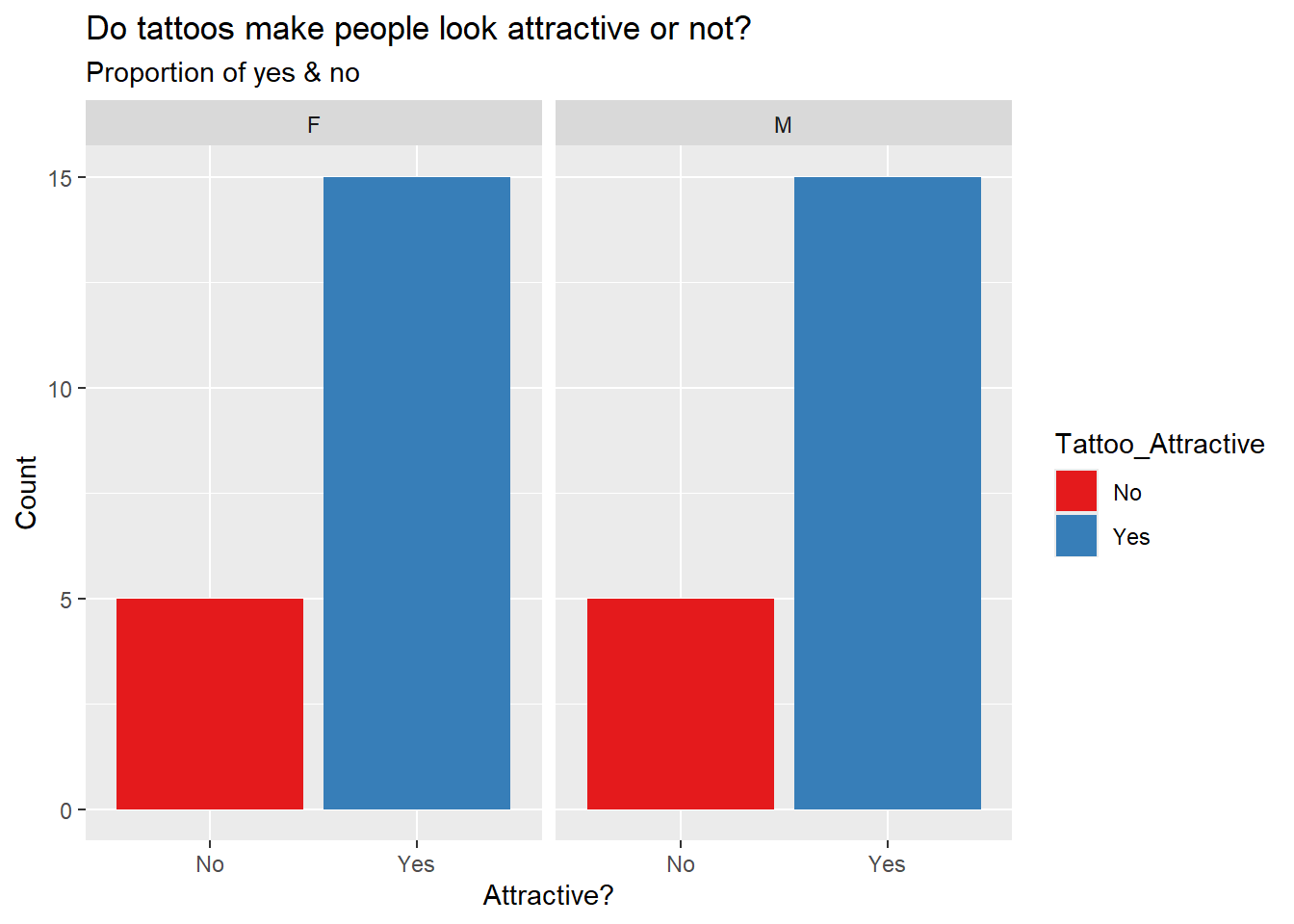
1 F      No                    5
2 F      Yes                  15
3 M      No                    5
4 M      Yes                  15

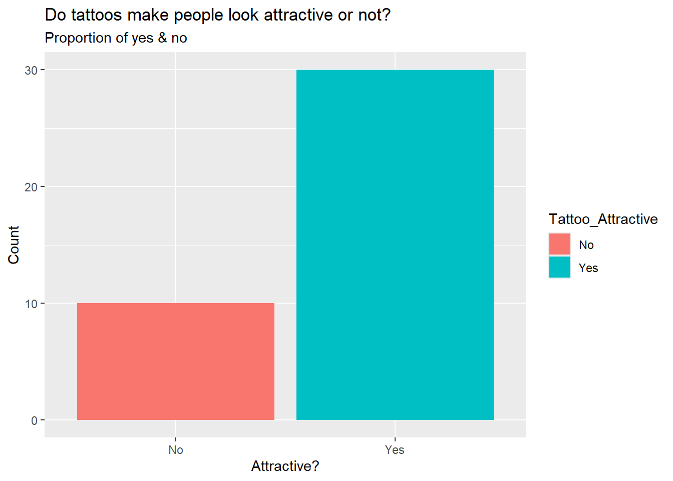
tat_modified %>%
  summarize(prop = prop(Tattoo_Attractive, success = "Yes"), n = n())

  prop  n
1 0.75 40

Visualising the Data

tat_modified %>%
  gf_bar(~Tattoo_Attractive, fill = ~ Tattoo_Attractive) %>%
  gf_labs(
    x = "Attractive?",
    y = "Count",
    title = "Do tattoos make people look attractive or not?",
    subtitle = "Proportion of yes & no"
  ) 

tat_modified %>%
  gf_bar(~Tattoo_Attractive | Gender, fill = ~ Tattoo_Attractive) %>%
  gf_labs(
    x = "Attractive?",
    y = "Count",
    title = "Do tattoos make people look attractive or not?",
    subtitle = "Proportion of yes & no"
  ) %>% 
  gf_refine(scale_fill_brewer(palette = "Set1"))

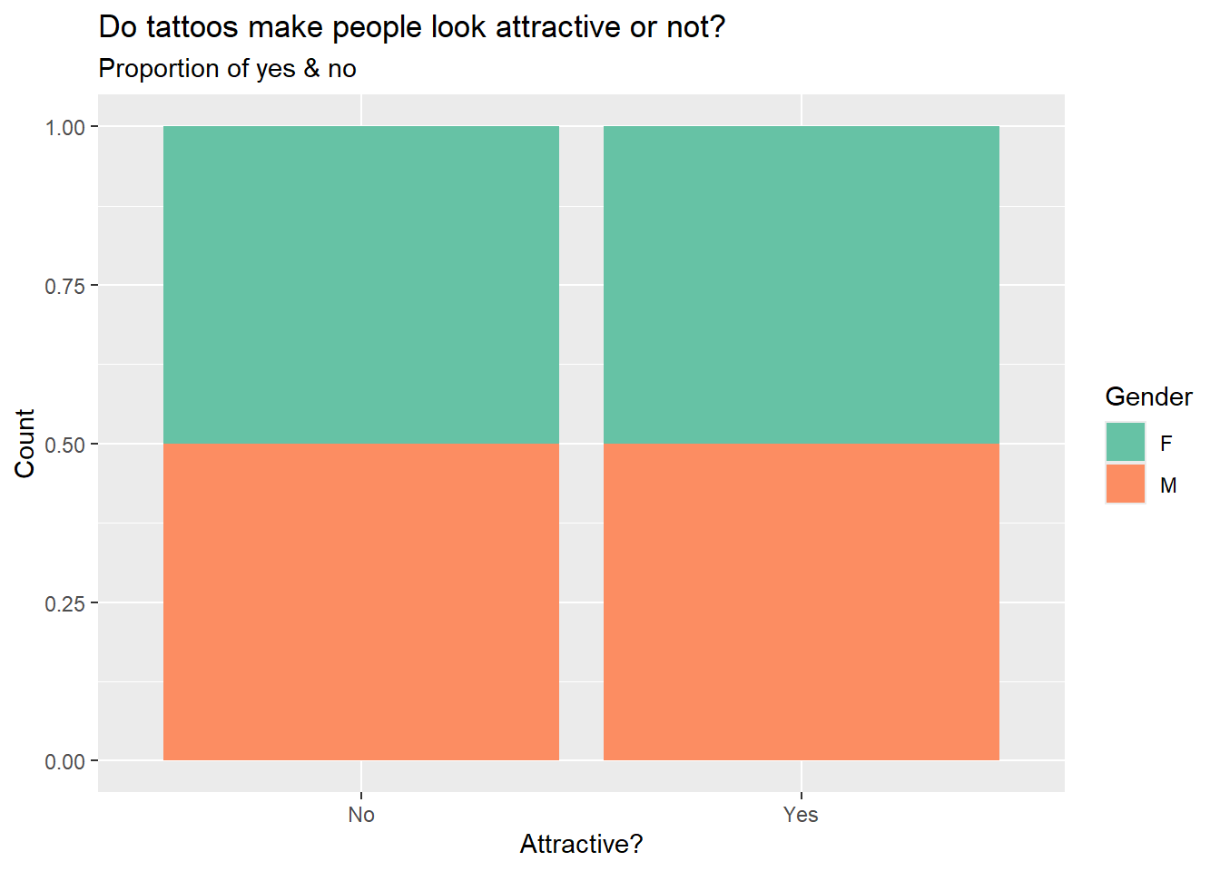
tat_modified %>%
  gf_bar(~Tattoo_Attractive, fill = ~ Gender, position = "fill") %>%
  gf_labs(
    x = "Attractive?",
    y = "Count",
    title = "Do tattoos make people look attractive or not?",
    subtitle = "Proportion of yes & no"
  ) %>% 
  gf_refine(scale_fill_brewer(palette = "Set2"))

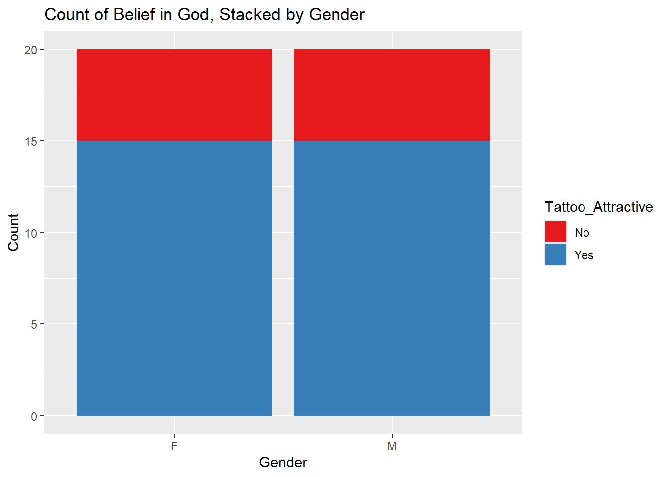
tat_modified %>%
  gf_bar(~Gender, fill = ~ Tattoo_Attractive, position = "stack") %>%
  gf_labs(
    x = "Gender",
    y = "Count",
    title = "Count of Belief in God, Stacked by Gender"
  ) %>%
  gf_refine(scale_fill_brewer(palette = "Set1"))

Prop Test: Does a majority of the population find tattoos attractive?

H0: p=0.5 (Half of the students think tattoos are attractive & Half of the students think tattoos are not attractive)

H1: p≠0.5

mosaic::binom.test(~Tattoo_Attractive, data = tat_modified, success = "Yes") %>% 
  broom::tidy()

# A tibble: 1 × 7
  estimate statistic p.value parameter conf.low conf.high alternative
     <dbl>     <dbl>   <dbl>     <dbl>    <dbl>     <dbl> <chr>      
1     0.75        30 0.00222        40    0.588     0.873 two.sided  

Inference:-

Since the p value <0.05, we reject the Null Hypothesis. Therefore, a high number of people find tattoos attractive (75%)

---

Chisq.test: Is there a difference in the proportion of males and females who find tattoos attractive?

H0: Proportion of males who find tattoos attractive is equal to the true proportion of females who find tattoos attractive.

H1: There is a difference between the proportion of males & females who find tattoos attractive.

contingency_table <- vcd::structable(Tattoo_Attractive~ Gender,
  data = tat_modified
)
contingency_table

       Tattoo_Attractive No Yes
Gender                         
F                         5  15
M                         5  15

gss_vcd_table <- vcd::structable(Tattoo_Attractive ~ Gender, data = tat_modified)
gss_vcd_table %>%
  vcd::mosaic(
    gp = shading_hsv, direction = "v",
    main = "Gender vs Tattoo Attractiveness",
    legend = TRUE,
    labeling = labeling_border(
      varnames = c("F", "F"), # Remove variable name labels
      rot_labels = c(90, 0, 0, 0), # t,r,b,l?
      just_labels = c(
        "left", # Top Side. How?
        "left", # Right side
        "left", # Bottom side
        "right"
      )
    )
  ) 

Warning in legend(residuals, gpfun, residuals_type): All residuals are zero.

Insight:

We see that from the plot above - all residuals are zero which confirms the null hypothesis that there isn’t a difference between both the groups.

xq_test_object <- chisq.test(contingency_table)
xq_test_object

    Pearson's Chi-squared test

data:  contingency_table
X-squared = 0, df = 1, p-value = 1

xq_test_object %>%
  broom::tidy() %>%
  select(statistic) %>%
  as.numeric() -> X_squared_observed
X_squared_observed

[1] 0

# Determine the Chi-Square critical value
X_squared_critical <- qchisq(
  p = .05,
  df = (2 - 1) * (2 - 1), # (nrows-1) * (ncols-1)
  lower.tail = FALSE
)
X_squared_critical

[1] 3.841459

mosaic::xqchisq(
  p = 0.95, df = 1,
  return = c("plot"), verbose = F,
  system = "gg"
) %>%
  gf_labs(
    x = "Chi-Square Value", 
    title = "Critical and Observed Chi-Square Values"
  ) %>%
  gf_vline(
    xintercept = X_squared_observed,
    color = "red", linewidth = 1
  ) %>%
  gf_vline(
    xintercept = X_squared_critical,
    color = "dodgerblue", linewidth = 1
  ) %>%
  gf_annotate(
    x = X_squared_observed + 0.2, y = 0.05,
    geom = "label", label = "Observed\nChi-Square",
    fill = "red", alpha = 0.3
  ) %>%
  gf_annotate(
    x = X_squared_critical - 0.5, y = 0.05,
    geom = "label", label = "Critical\nChi-Square",
    fill = "lightblue"
  )

Inference:-

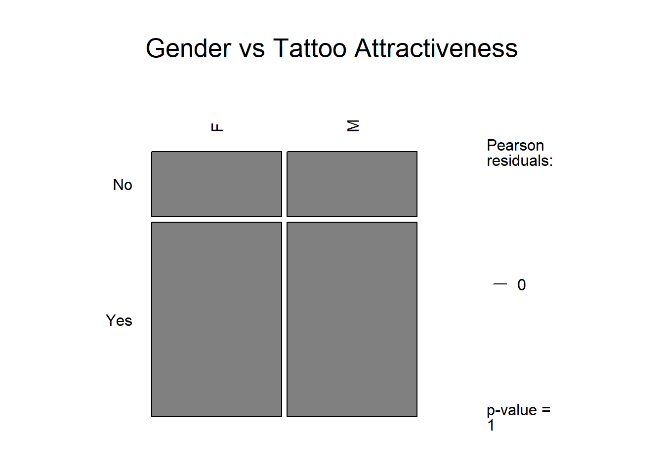
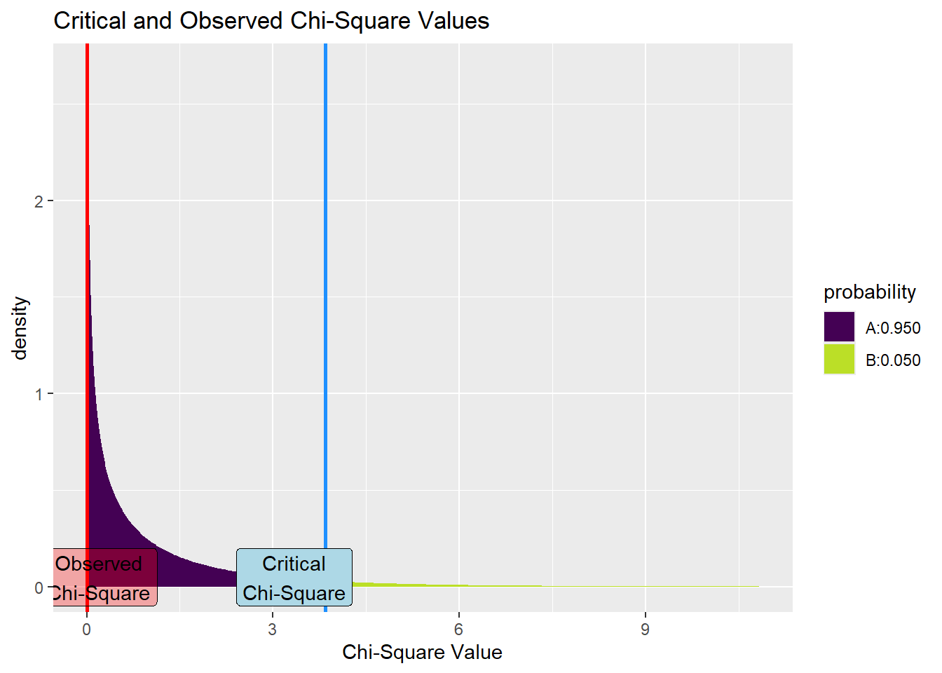
Since the observed value is less than the critical value and the p-value is greater than 0.05, we fail to reject the null hypothesis.

There is no significant difference between male and female respondents in how they perceive tattoos. Both genders gave almost identical responses which suggests that gender does not play a major role in determining whether tattoos are attractive or not.

Conclusion

To sum up, most of the people found tattoos attractive (75%). The proportion test confirmed that it is statistically significant. A chi-square test was conducted to see if opinions differ from men to women. The test showed no significant difference as both males and females gave the same responses. Overall, we see that tattoos are found attractive and gender doesn’t play a role in how it’s perceived.

---