Is the average weekly expenditure for boys equal to girls?
Author
Diya Bijoy
Published
November 4, 2025
R Packages Setup
library(tidyverse)
── Attaching core tidyverse packages ──────────────────────── tidyverse 2.0.0 ──
✔ dplyr     1.1.4     ✔ readr     2.1.5
✔ forcats   1.0.0     ✔ stringr   1.5.1
✔ ggplot2   4.0.0     ✔ tibble    3.3.0
✔ lubridate 1.9.4     ✔ tidyr     1.3.1
✔ purrr     1.1.0
── Conflicts ────────────────────────────────────────── tidyverse_conflicts() ──
✖ dplyr::filter() masks stats::filter()
✖ dplyr::lag()    masks stats::lag()
ℹ Use the conflicted package (<http://conflicted.r-lib.org/>) to force all conflicts to become errors
library(mosaic)
Registered S3 method overwritten by 'mosaic':
  method                           from
  fortify.SpatialPolygonsDataFrame ggplot2

The 'mosaic' package masks several functions from core packages in order to add
additional features.  The original behavior of these functions should not be affected by this.

Attaching package: 'mosaic'

The following object is masked from 'package:Matrix':

    mean

The following objects are masked from 'package:dplyr':

    count, do, tally

The following object is masked from 'package:purrr':

    cross

The following object is masked from 'package:ggplot2':

    stat

The following objects are masked from 'package:stats':

    binom.test, cor, cor.test, cov, fivenum, IQR, median, prop.test,
    quantile, sd, t.test, var

The following objects are masked from 'package:base':

    max, mean, min, prod, range, sample, sum
library(ggformula)library(infer)
Attaching package: 'infer'

The following objects are masked from 'package:mosaic':

    prop_test, t_test
library(broom) # Clean test results in tibble formlibrary(resampledata) # Datasets from Chihara and Hesterberg's book
Attaching package: 'resampledata'

The following object is masked from 'package:datasets':

    Titanic
library(openintro) # More datasets
Loading required package: airports
Loading required package: cherryblossom
Loading required package: usdata

Attaching package: 'openintro'

The following object is masked from 'package:mosaic':

    dotPlot

The following objects are masked from 'package:lattice':

    ethanol, lsegments
library(visStatistics) # One package to rule them alllibrary(ggstatsplot)
You can cite this package as:
     Patil, I. (2021). Visualizations with statistical details: The 'ggstatsplot' approach.
     Journal of Open Source Software, 6(61), 3167, doi:10.21105/joss.03167
    Shapiro-Wilk normality test

data:  girls_expense$Total_Expenditure_Last_Week
W = 0.78317, p-value = 0.0004899
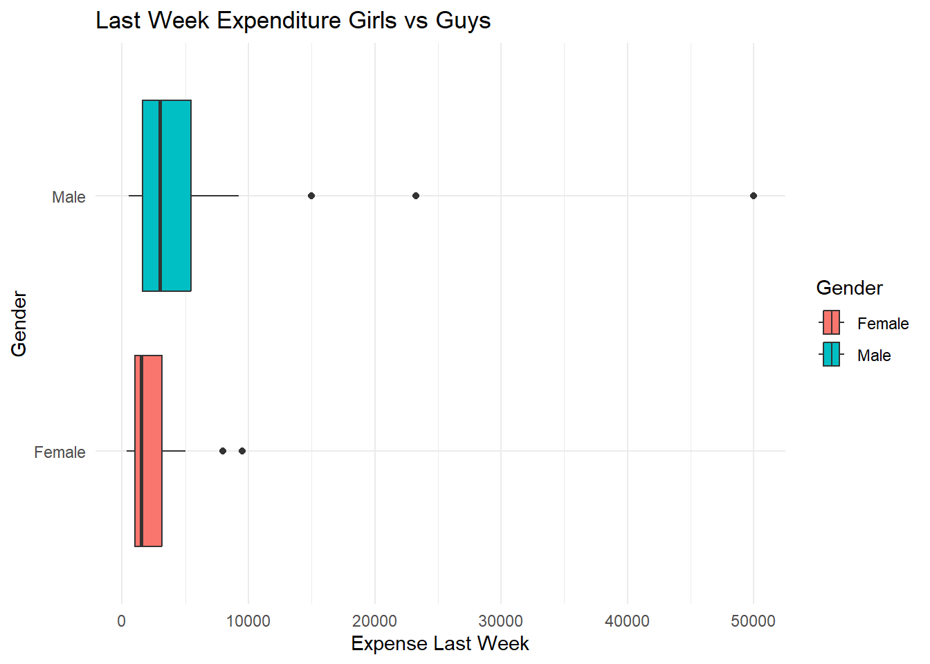
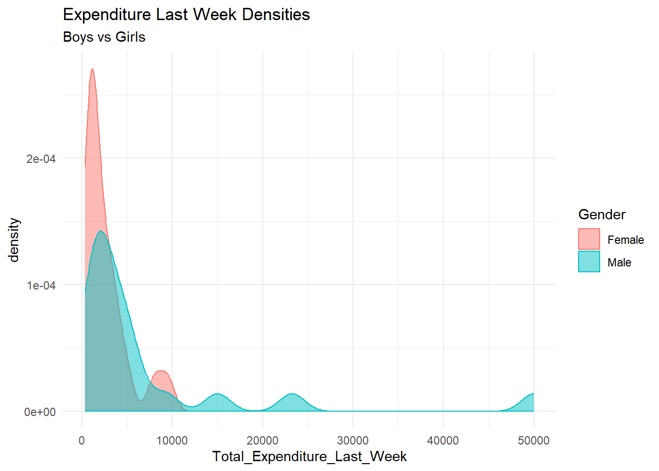
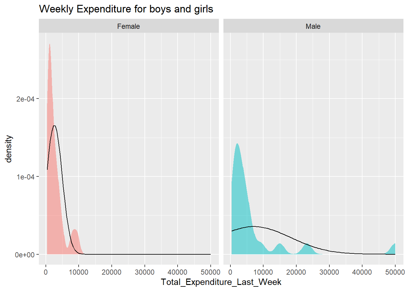
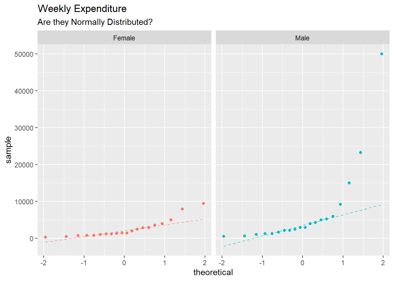
P value for both boys & girls is less than 0.05, therefore its not normally distributed. This means that the distributions of weekly expenditure for both boys and girls deviate significantly from a normal distribution.
The variance is way off with a p value 8.53 * 10^-9 which is much less than 0.05, so therefore the variance for the variables is significantly different.
Inference
The two variables are not normally distributed.
The two variances are also significantly different.
This means that its Non-Parametric so the Mann-Whitney Test & Permutation Test must be done since its not normally distributed and the variances is different.
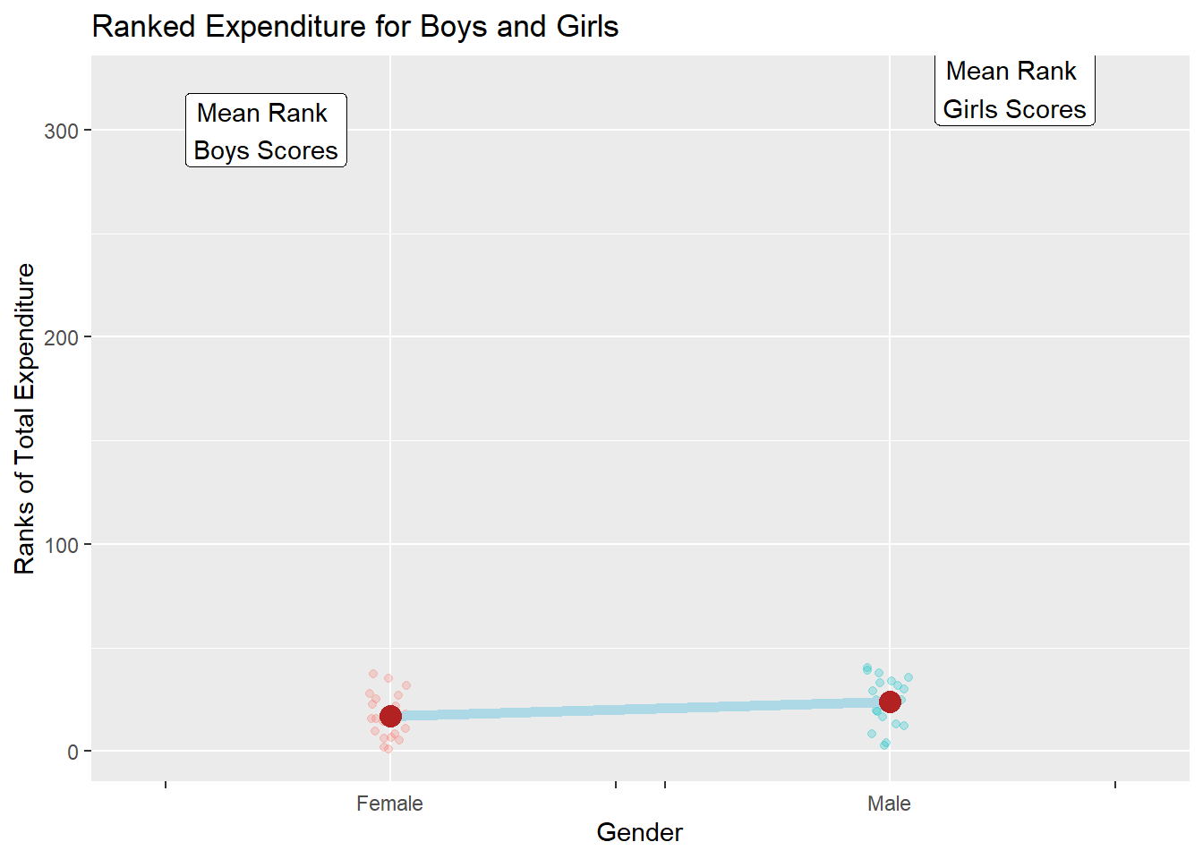
1. Mann-Whitney Test
H0: The rank sums for girls and boys do not differ significantly.
H1: The rank sums for girls and boys do differ significantly.
library(ggprism)library(ggtext)library(glue)library(latex2exp)exp_modified %>%gf_jitter(rank(Total_Expenditure_Last_Week) ~ Gender,color =~Gender,show.legend =FALSE,width =0.05, alpha =0.25,ylab ="Ranks of Total Expenditure",title ="Ranked Expenditure for Boys and Girls" ) %>%gf_summary(group =~1, fun ="mean", geom ="line", colour ="lightblue",lty =1, linewidth =2 ) %>%gf_summary(fun ="mean", colour ="firebrick", size =4, geom ="point") %>%gf_refine(scale_x_discrete(breaks =c("Male", "Female"),labels =c("Male", "Female"),guide ="prism_bracket" )) %>%gf_annotate("label",label ="Mean Rank \nBoys Scores",y =300, x =0.75, inherit =FALSE ) %>%gf_annotate("label",label ="Mean Rank \nGirls Scores",y =320, x =2.25, inherit =FALSE )
Warning in ggplot2::annotate(geom = geom, x = x, y = y, xmin = xmin, xmax = xmax, : Ignoring unknown parameters: `inherit`
Ignoring unknown parameters: `inherit`
Warning: The S3 guide system was deprecated in ggplot2 3.5.0.
ℹ It has been replaced by a ggproto system that can be extended.
Here, we see that the p value = 0.06 which is >0.05, so we fail to reject the Null Hypothesis. This means there is no statistically significant difference in weekly expenditure between boys and girls.
The p-value was 0.06, which is slightly greater than the 0.05 threshold.
We fail to reject the null hypothesis, which means that there is no statistically significant difference in the distribution of weekly expenditure between boys and girls.
null_dist_infer %>%get_p_value(obs_stat = obs_diff_infer, direction ="two-sided")
# A tibble: 1 × 1
  p_value
    <dbl>
1  0.0556
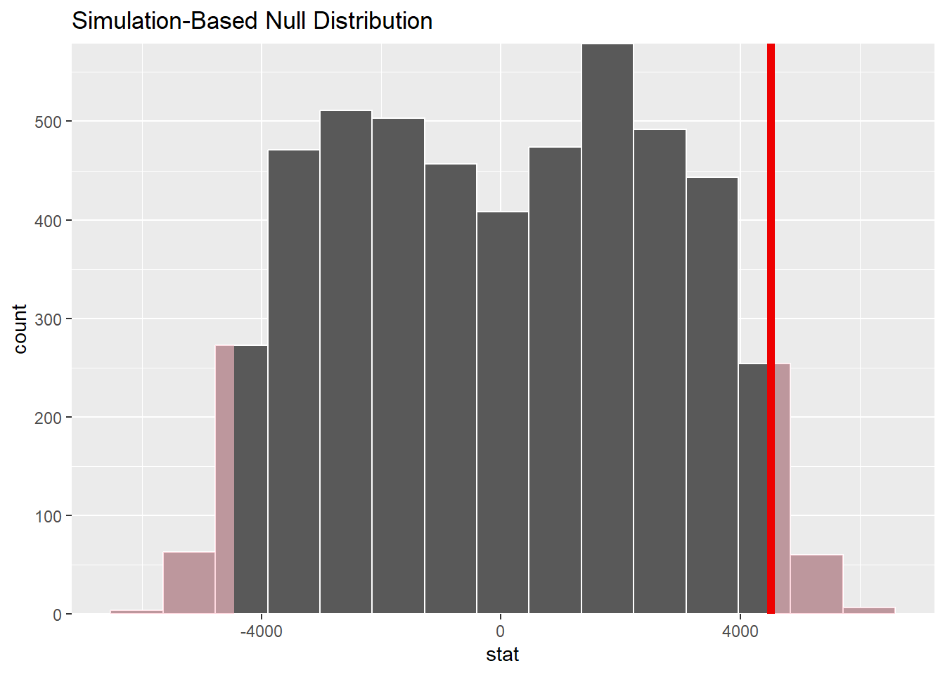
Inferences:-
The p value = 0.059 (5.9%), which is greater than the 0.05 threshold.
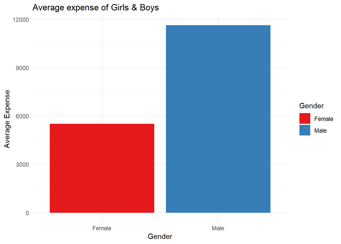
So we fail to reject the Null Hypothesis that weekly expenditure is independent of gender. So the observed difference of Rs. 4502.75 has occurred due to random chance.
Conclusion
To conclude, while boys appear to have spent a bit more on average than girls, statistical tests show that this difference is not significant. Both the Mann Whitney and permutation tests indicate that gender does not play a major role in determining weekly spending. Overall, weekly expenditure patterns are fairly similar between boys and girls.