New to ggformula?  Try the tutorials:
    learnr::run_tutorial("introduction", package = "ggformula")
    learnr::run_tutorial("refining", package = "ggformula")
library(janitor)
Attaching package: 'janitor'
The following objects are masked from 'package:stats':

    chisq.test, fisher.test
library(mosaic)
Registered S3 method overwritten by 'mosaic':
  method                           from
  fortify.SpatialPolygonsDataFrame ggplot2
The 'mosaic' package masks several functions from core packages in order to add
additional features.  The original behavior of these functions should not be affected by this.
Attaching package: 'mosaic'
The following objects are masked from 'package:dplyr':

    count, do, tally
The following object is masked from 'package:Matrix':

    mean
The following object is masked from 'package:scales':

    rescale
The following object is masked from 'package:ggplot2':

    stat
The following objects are masked from 'package:stats':

    binom.test, cor, cor.test, cov, fivenum, IQR, median, prop.test,
    quantile, sd, t.test, var
The following objects are masked from 'package:base':

    max, mean, min, prod, range, sample, sum
library(naniar)library(skimr)
Attaching package: 'skimr'
The following object is masked from 'package:naniar':

    n_complete
The following object is masked from 'package:mosaic':

    n_missing
Attaching package: 'infer'

The following objects are masked from 'package:mosaic':

    prop_test, t_test
library(resampledata)
Attaching package: 'resampledata'

The following object is masked from 'package:datasets':

    Titanic
library(openintro)
Loading required package: airports
Loading required package: cherryblossom
Loading required package: usdata

Attaching package: 'openintro'

The following object is masked from 'package:GGally':

    tips

The following object is masked from 'package:mosaic':

    dotPlot

The following objects are masked from 'package:lattice':

    ethanol, lsegments
library(vcd)
Loading required package: grid

Attaching package: 'vcd'

The following object is masked from 'package:mosaic':

    mplot
Rows: 65
Columns: 4
$ name         <fct> Manya, Sradha, Arun, Nidhi, Shaurya, Pratham, Jeevan, Dhr…
$ gender       <fct> F, F, M, F, M, M, M, M, F, M, F, M, F, F, M, M, F, M, M, …
$ college      <fct> SMI, SMI, SMI, SMI, MIT, MIT, MIT, SMI, SMI, SMI, SMI, SM…
$ is_dad_weird <fct> No, No, No, Yes, No, No, No, No, Yes, Yes, Yes, Yes, No, …
# A tibble: 5 × 3
# Groups:   gender [3]
  gender is_dad_weird     n
  <fct>  <fct>        <int>
1 F      No              23
2 F      Yes              9
3 M      No              24
4 M      Yes              7
5 NB     Yes              1
Visualising the Data
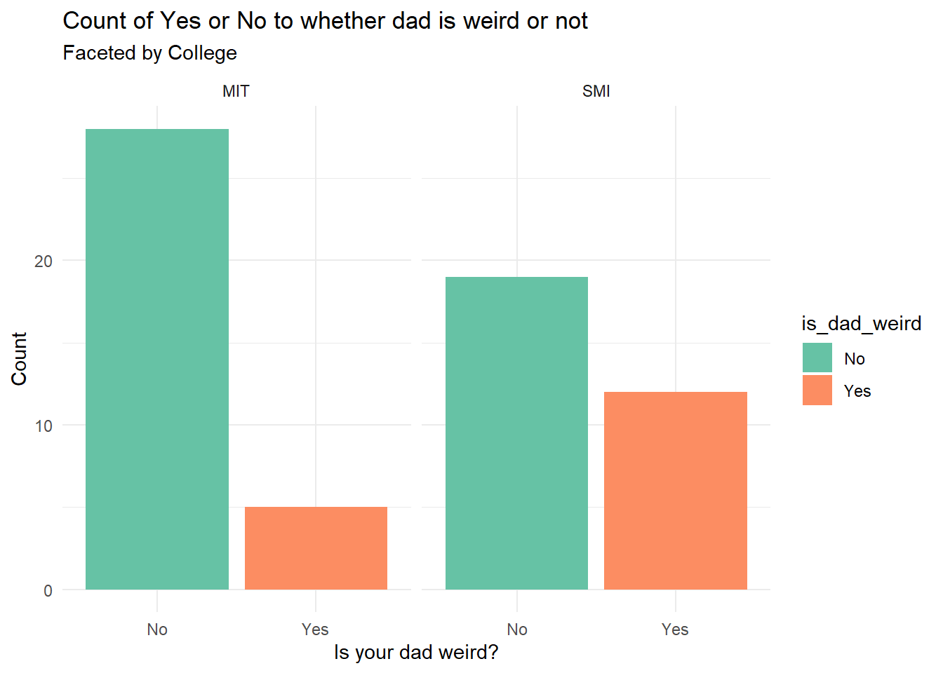
weird_dads_modified2 %>%gf_bar(~is_dad_weird | college, fill =~ is_dad_weird) %>%gf_labs(title ="Count of Yes or No to whether dad is weird or not",subtitle ="Faceted by College",x ="Is your dad weird?",y ="Count" ) %>%gf_refine(scale_fill_brewer(palette ="Set2")) %>%gf_theme(theme_minimal)
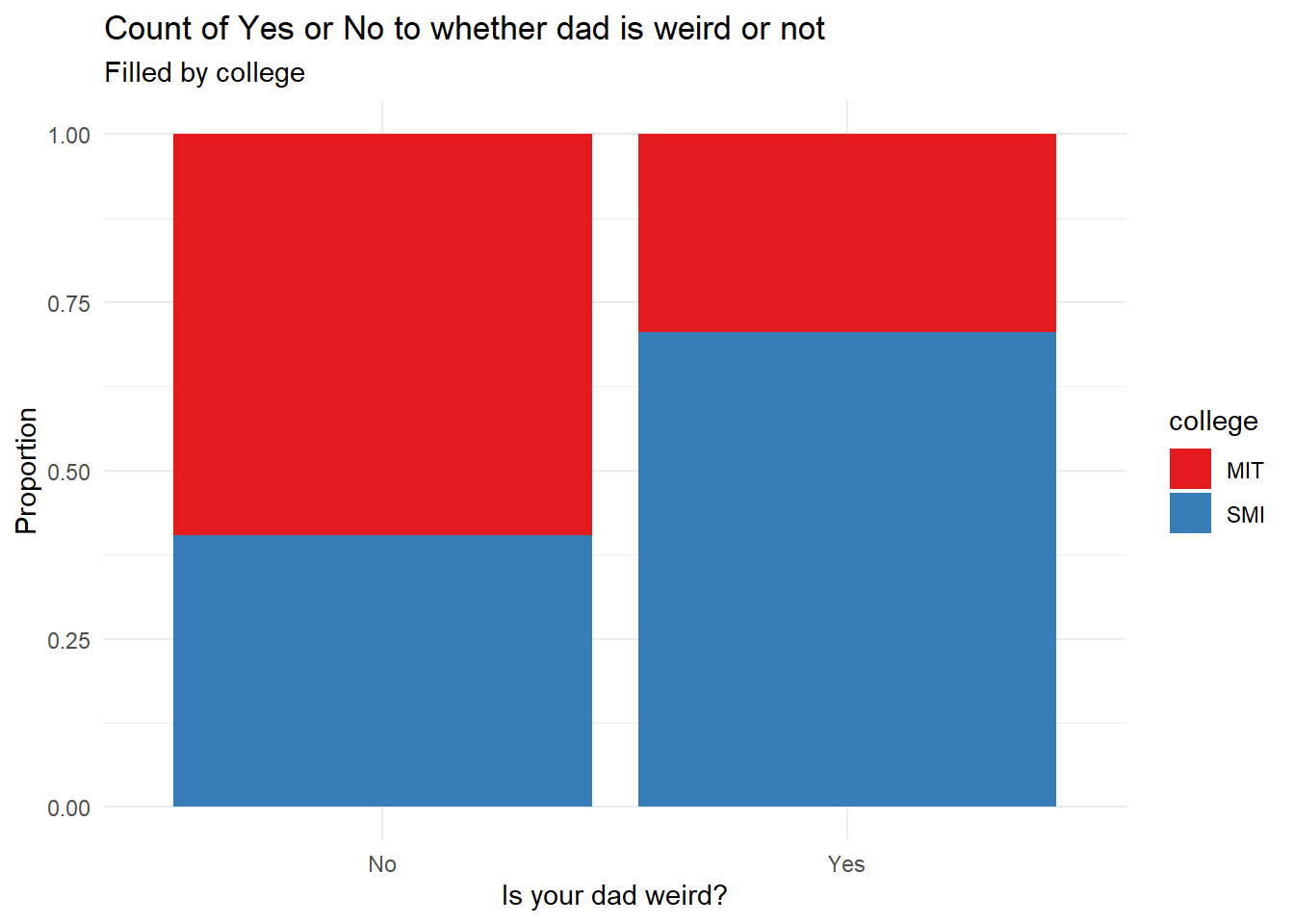
weird_dads_modified2 %>%gf_bar(~is_dad_weird, fill =~ college, position ="fill") %>%gf_labs(title ="Count of Yes or No to whether dad is weird or not",subtitle ="Filled by college",x ="Is your dad weird?",y ="Proportion" ) %>%gf_refine(scale_fill_brewer(palette ="Set1")) %>%gf_theme(theme_minimal)
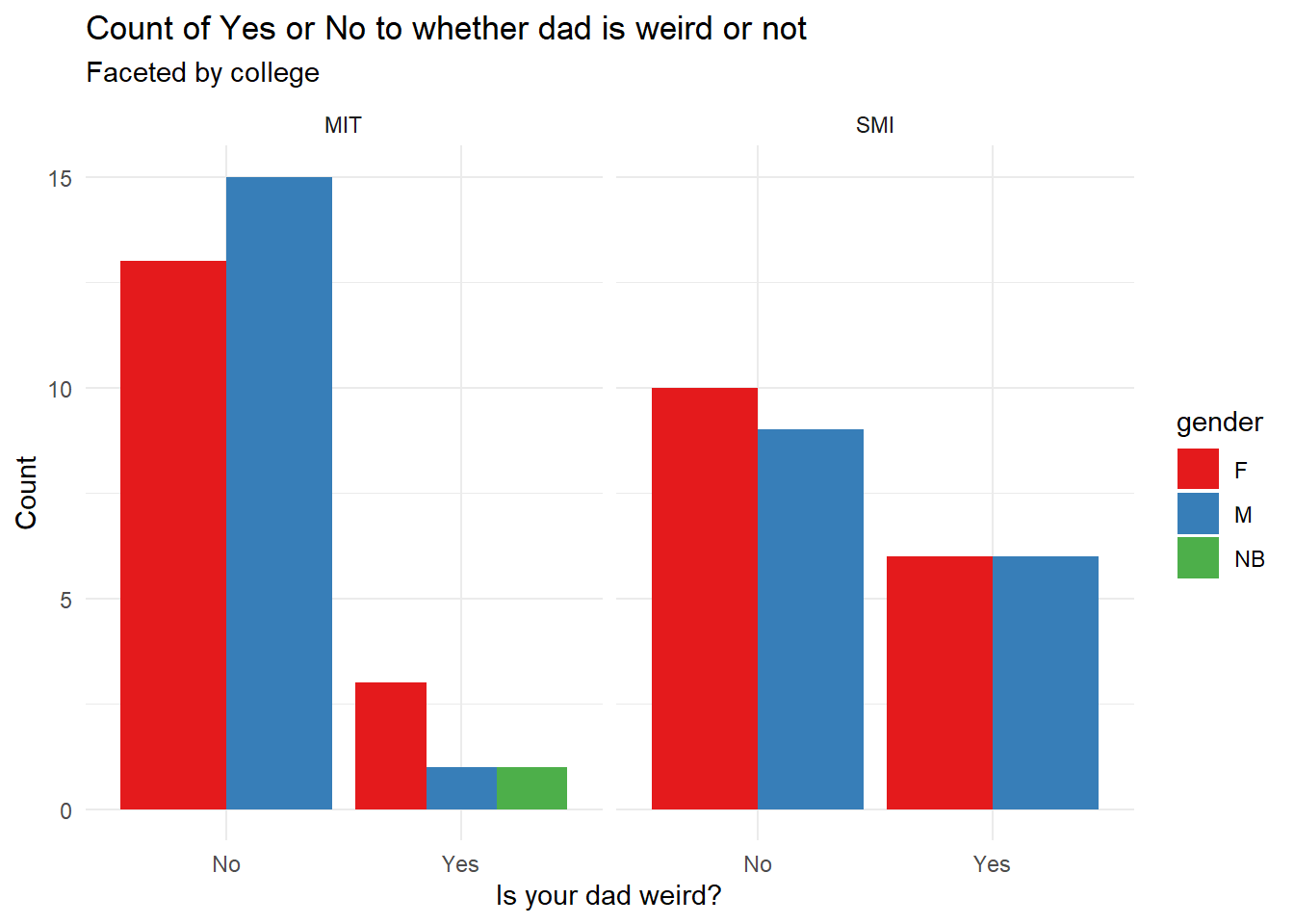
weird_dads_modified2 %>%gf_bar(~is_dad_weird | college, fill =~ gender, position ="dodge") %>%gf_labs(title ="Count of Yes or No to whether dad is weird or not",subtitle ="Faceted by college",x ="Is your dad weird?",y ="Count" ) %>%gf_refine(scale_fill_brewer(palette ="Set1")) %>%gf_theme(theme_minimal)
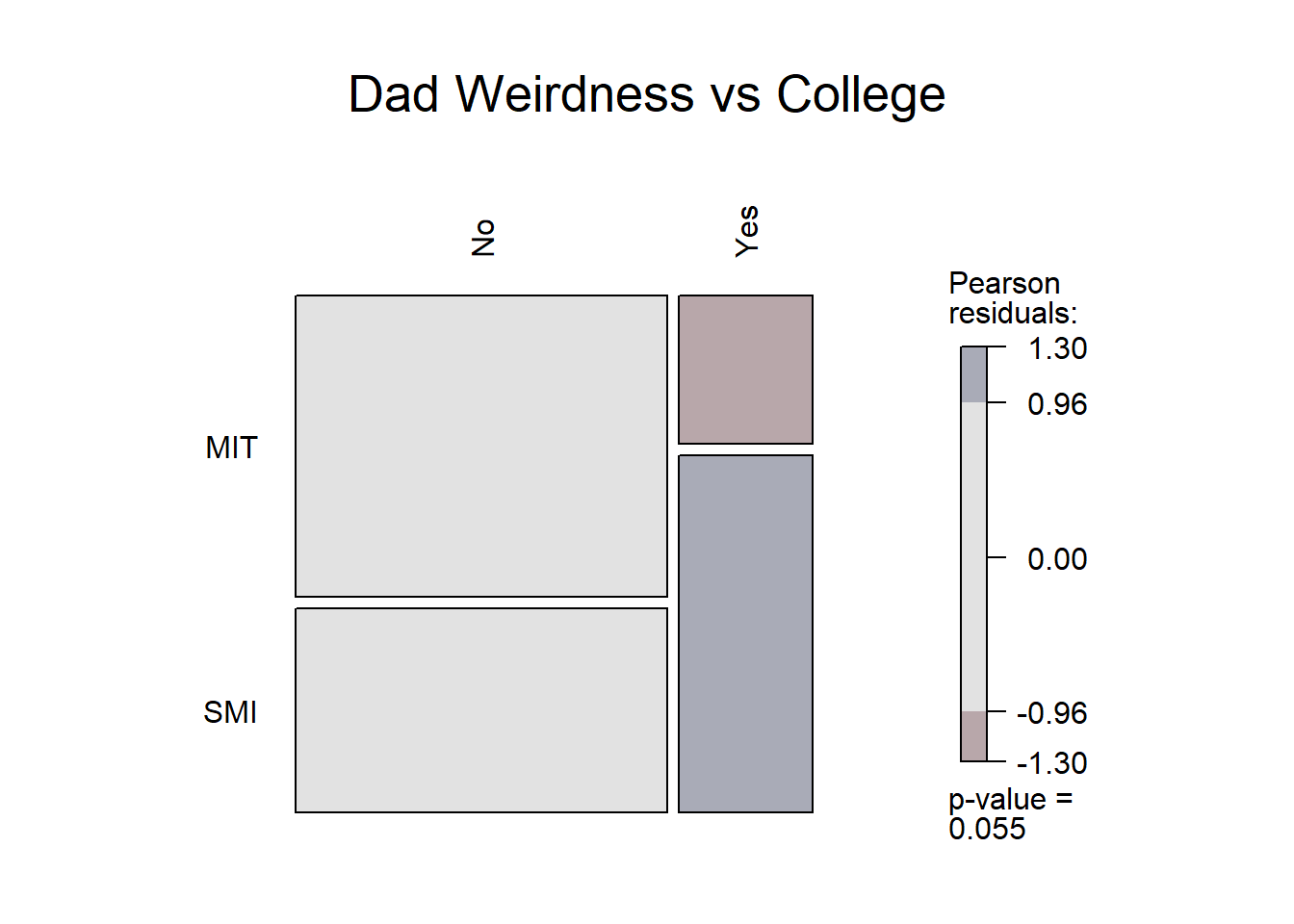
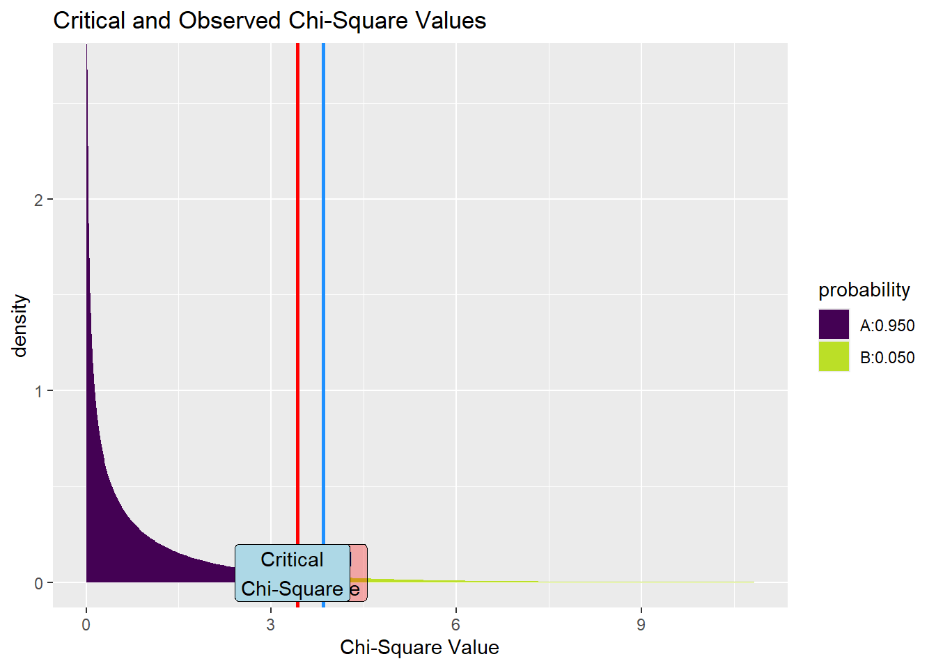
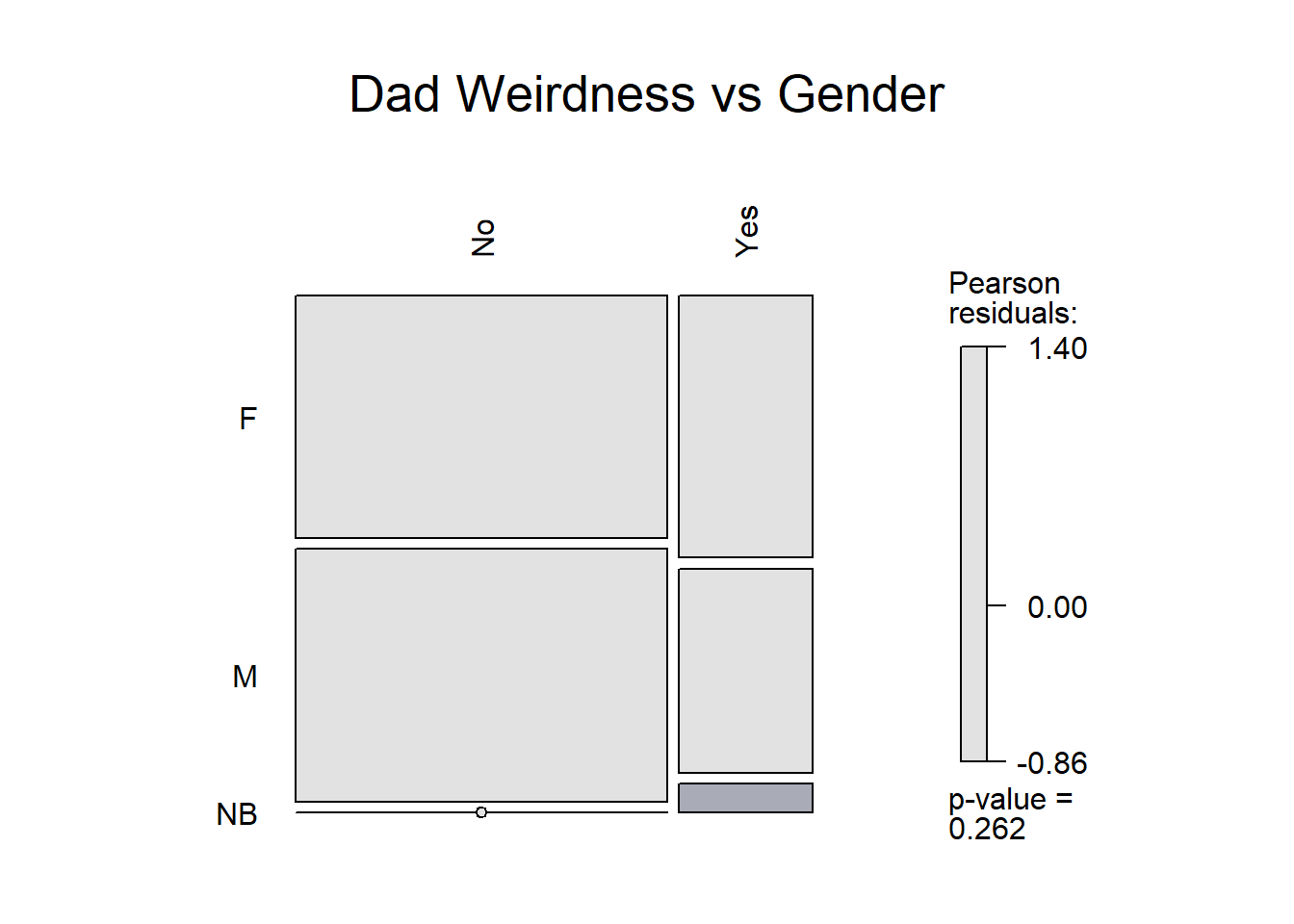
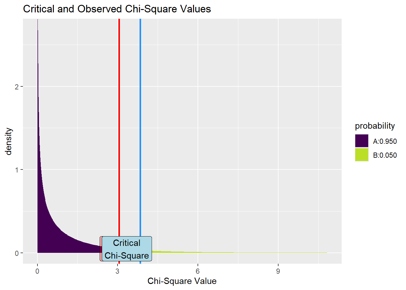
To conclude, chi-square tests indicate that neither college nor gender significantly affect perceptions of dad weirdness. Overall, the hunch that “Srishti dads are weird” is not statistically supported - dads in MIT & SMI seem to have a similar level of weirdness.