Classwork 9

library(tidyverse)

── Attaching core tidyverse packages ──────────────────────── tidyverse 2.0.0 ──
✔ dplyr     1.1.4     ✔ readr     2.1.5
✔ forcats   1.0.0     ✔ stringr   1.5.1
✔ ggplot2   4.0.0     ✔ tibble    3.3.0
✔ lubridate 1.9.4     ✔ tidyr     1.3.1
✔ purrr     1.1.0     
── Conflicts ────────────────────────────────────────── tidyverse_conflicts() ──
✖ dplyr::filter() masks stats::filter()
✖ dplyr::lag()    masks stats::lag()
ℹ Use the conflicted package (<http://conflicted.r-lib.org/>) to force all conflicts to become errors

library(mosaic)

Registered S3 method overwritten by 'mosaic':
  method                           from   
  fortify.SpatialPolygonsDataFrame ggplot2

The 'mosaic' package masks several functions from core packages in order to add 
additional features.  The original behavior of these functions should not be affected by this.

Attaching package: 'mosaic'

The following object is masked from 'package:Matrix':

    mean

The following objects are masked from 'package:dplyr':

    count, do, tally

The following object is masked from 'package:purrr':

    cross

The following object is masked from 'package:ggplot2':

    stat

The following objects are masked from 'package:stats':

    binom.test, cor, cor.test, cov, fivenum, IQR, median, prop.test,
    quantile, sd, t.test, var

The following objects are masked from 'package:base':

    max, mean, min, prod, range, sample, sum

library(ggformula)
library(infer)

Attaching package: 'infer'

The following objects are masked from 'package:mosaic':

    prop_test, t_test

## Datasets from Chihara and Hesterberg's book (Second Edition)
library(resampledata)

Attaching package: 'resampledata'

The following object is masked from 'package:datasets':

    Titanic

## Datasets from Cetinkaya-Rundel and Hardin's book (First Edition)
library(openintro)

Loading required package: airports
Loading required package: cherryblossom
Loading required package: usdata

Attaching package: 'openintro'

The following object is masked from 'package:mosaic':

    dotPlot

The following objects are masked from 'package:lattice':

    ethanol, lsegments

data(yrbss, package = "openintro")
yrbss

# A tibble: 13,583 × 13
     age gender grade hispanic race                     height weight helmet_12m
   <int> <chr>  <chr> <chr>    <chr>                     <dbl>  <dbl> <chr>     
 1    14 female 9     not      Black or African Americ…  NA      NA   never     
 2    14 female 9     not      Black or African Americ…  NA      NA   never     
 3    15 female 9     hispanic Native Hawaiian or Othe…   1.73   84.4 never     
 4    15 female 9     not      Black or African Americ…   1.6    55.8 never     
 5    15 female 9     not      Black or African Americ…   1.5    46.7 did not r…
 6    15 female 9     not      Black or African Americ…   1.57   67.1 did not r…
 7    15 female 9     not      Black or African Americ…   1.65  132.  did not r…
 8    14 male   9     not      Black or African Americ…   1.88   71.2 never     
 9    15 male   9     not      Black or African Americ…   1.75   63.5 never     
10    15 male   10    not      Black or African Americ…   1.37   97.1 did not r…
# ℹ 13,573 more rows
# ℹ 5 more variables: text_while_driving_30d <chr>, physically_active_7d <int>,
#   hours_tv_per_school_day <chr>, strength_training_7d <int>,
#   school_night_hours_sleep <chr>

yrbss %>%
  group_by(helmet_12m) %>%
  count()

# A tibble: 7 × 2
# Groups:   helmet_12m [7]
  helmet_12m       n
  <chr>        <int>
1 always         399
2 did not ride  4549
3 most of time   293
4 never         6977
5 rarely         713
6 sometimes      341
7 <NA>           311

yrbss %>%
  group_by(text_while_driving_30d) %>%
  count()

# A tibble: 9 × 2
# Groups:   text_while_driving_30d [9]
  text_while_driving_30d     n
  <chr>                  <int>
1 0                       4792
2 1-2                      925
3 10-19                    373
4 20-29                    298
5 3-5                      493
6 30                       827
7 6-9                      311
8 did not drive           4646
9 <NA>                     918

no_helmet_text <- yrbss %>%
  filter(helmet_12m == "never") %>%
  mutate(text_ind = ifelse(text_while_driving_30d == "30", "yes", "no")) %>%
  # removing most of the other variables
  select(age, gender, text_ind)
no_helmet_text

# A tibble: 6,977 × 3
     age gender text_ind
   <int> <chr>  <chr>   
 1    14 female no      
 2    14 female <NA>    
 3    15 female yes     
 4    15 female no      
 5    14 male   <NA>    
 6    15 male   <NA>    
 7    16 male   no      
 8    14 male   no      
 9    15 male   no      
10    16 male   no      
# ℹ 6,967 more rows

no_helmet_text %>%
  drop_na() %>%
  count(text_ind)

# A tibble: 2 × 2
  text_ind     n
  <chr>    <int>
1 no        6025
2 yes        462

no_helmet_text %>%
  drop_na() %>%
  summarize(prop = prop(text_ind, success = "yes"), n = n())

# A tibble: 1 × 2
    prop     n
   <dbl> <int>
1 0.0712  6487

no_helmet_text %>%
  drop_na() %>%
  gf_bar(~text_ind) %>%
  gf_labs(
    x = "texted?",
    title = "High-Schoolers who texted every day",
    subtitle = "While driving with no helmet on!!"
  )

mosaic::binom.test(~text_ind, data = no_helmet_text, success = "yes")

data:  no_helmet_text$text_ind  [with success = yes]
number of successes = 463, number of trials = 6503, p-value < 2.2e-16
alternative hypothesis: true probability of success is not equal to 0.5
95 percent confidence interval:
 0.06506429 0.07771932
sample estimates:
probability of success 
            0.07119791 

mosaic::binom.test(~text_ind, data = no_helmet_text, success = "yes") %>%
  broom::tidy()

# A tibble: 1 × 7
  estimate statistic p.value parameter conf.low conf.high alternative
     <dbl>     <dbl>   <dbl>     <dbl>    <dbl>     <dbl> <chr>      
1   0.0712       463       0      6503   0.0651    0.0777 two.sided  

---

Multiple Proportions

data(GSS2002, package = "resampledata")
glimpse(GSS2002)

Rows: 2,765
Columns: 21
$ ID            <int> 1, 2, 3, 4, 5, 6, 7, 8, 9, 10, 11, 12, 13, 14, 15, 16, 1…
$ Region        <fct> South Central, South Central, South Central, South Centr…
$ Gender        <fct> Female, Male, Female, Female, Male, Male, Female, Female…
$ Race          <fct> White, White, White, White, White, White, White, White, …
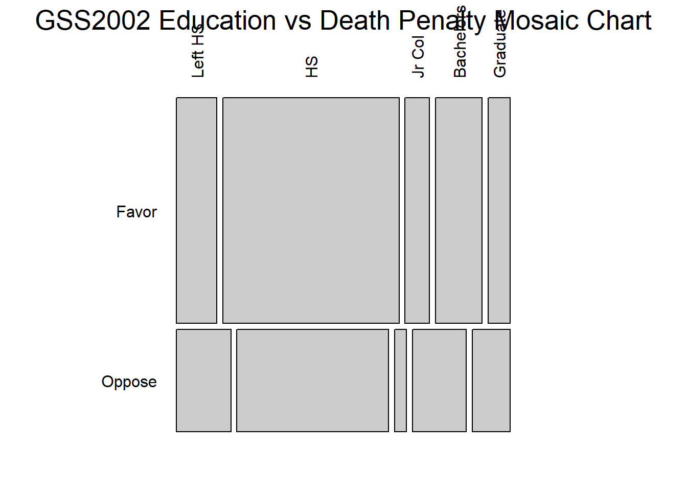
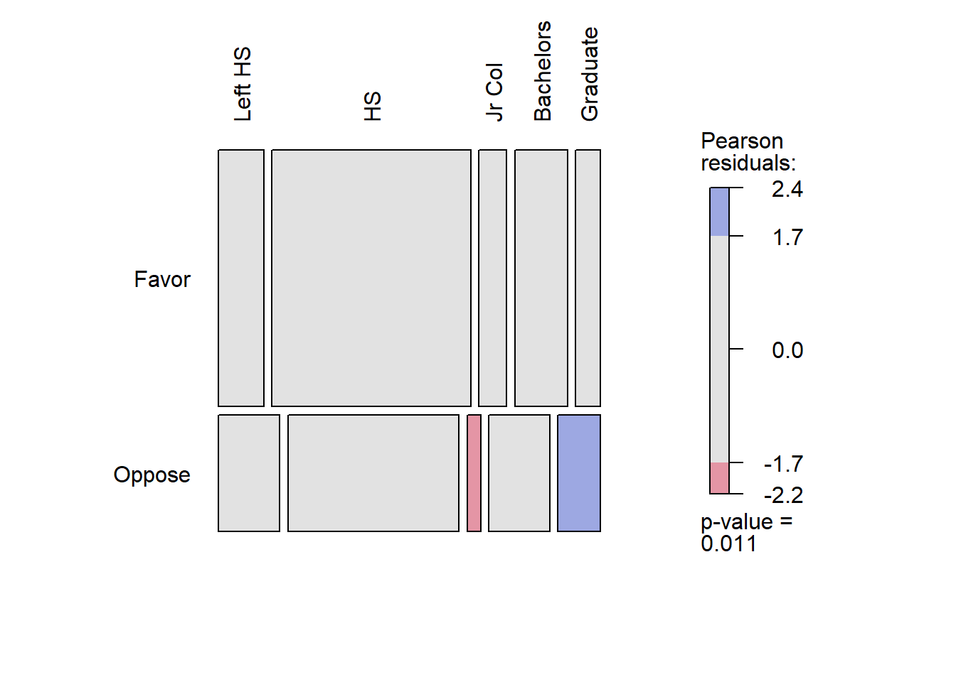
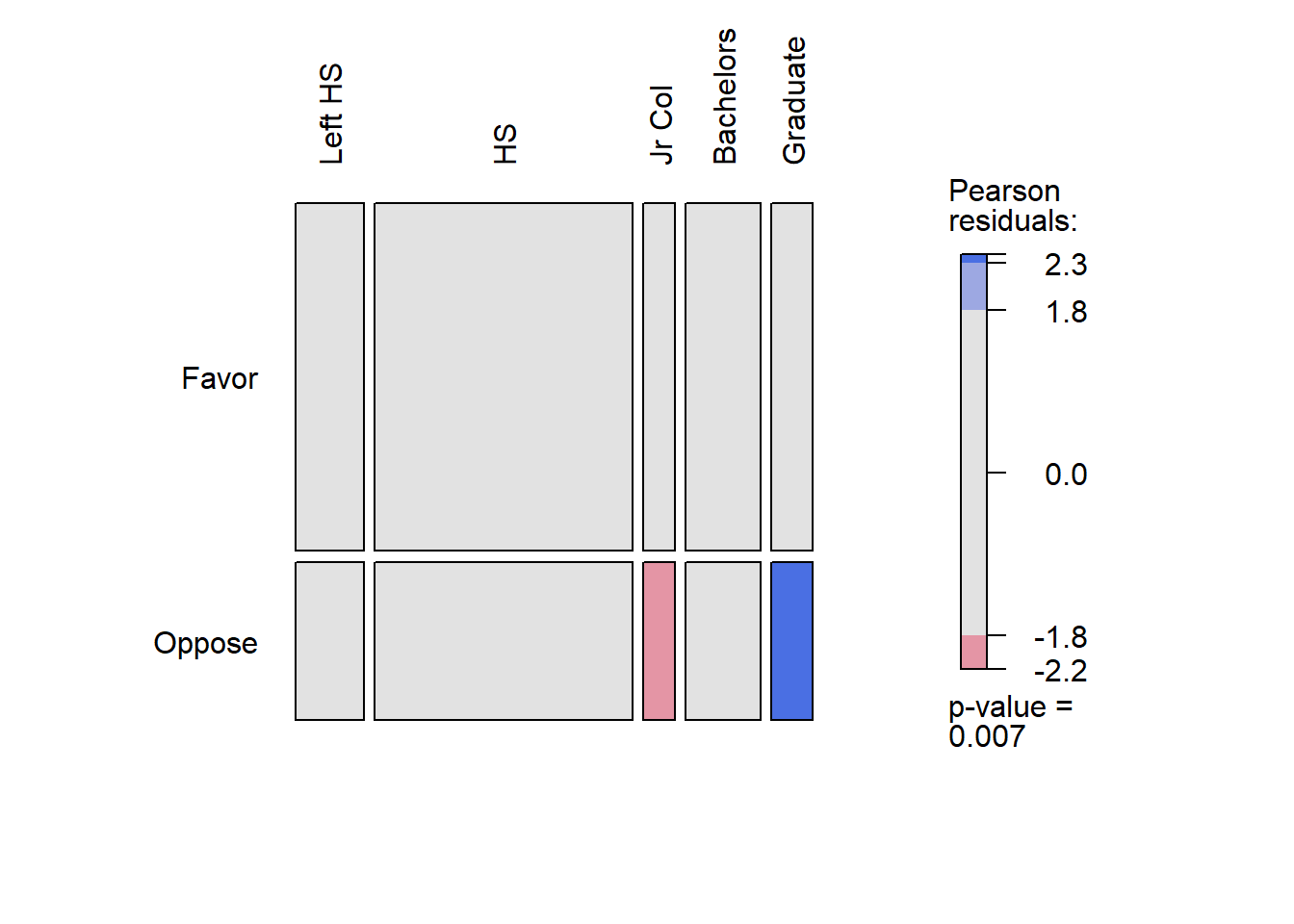
$ Education     <fct> HS, Bachelors, HS, Left HS, Left HS, HS, Bachelors, HS, …
$ Marital       <fct> Divorced, Married, Separated, Divorced, Divorced, Divorc…
$ Religion      <fct> Inter-nondenominational, Protestant, Protestant, Protest…
$ Happy         <fct> Pretty happy, Pretty happy, NA, NA, NA, Pretty happy, NA…
$ Income        <fct> 30000-34999, 75000-89999, 35000-39999, 50000-59999, 4000…
$ PolParty      <fct> "Strong Rep", "Not Str Rep", "Strong Rep", "Ind, Near De…
$ Politics      <fct> Conservative, Conservative, NA, NA, NA, Conservative, NA…
$ Marijuana     <fct> NA, Not legal, NA, NA, NA, NA, NA, NA, Legal, NA, NA, NA…
$ DeathPenalty  <fct> Favor, Favor, NA, NA, NA, Favor, NA, NA, Favor, NA, NA, …
$ OwnGun        <fct> No, Yes, NA, NA, NA, Yes, NA, NA, Yes, NA, NA, NA, NA, N…
$ GunLaw        <fct> Favor, Oppose, NA, NA, NA, Oppose, NA, NA, Oppose, NA, N…
$ SpendMilitary <fct> Too little, About right, NA, About right, NA, Too little…
$ SpendEduc     <fct> Too little, Too little, NA, Too little, NA, Too little, …
$ SpendEnv      <fct> About right, About right, NA, Too little, NA, Too little…
$ SpendSci      <fct> About right, About right, NA, Too little, NA, Too little…
$ Pres00        <fct> Bush, Bush, Bush, NA, NA, Bush, Bush, Bush, Bush, NA, NA…
$ Postlife      <fct> Yes, Yes, NA, NA, NA, Yes, NA, NA, Yes, NA, NA, NA, NA, …

GSS2002 %>% count(Education)

  Education    n
1   Left HS  400
2        HS 1485
3    Jr Col  202
4 Bachelors  443
5  Graduate  230
6      <NA>    5

GSS2002 %>% count(DeathPenalty)

  DeathPenalty    n
1        Favor  899
2       Oppose  409
3         <NA> 1457

GSS2002_modified <- GSS2002 %>%
  dplyr::select(Education, DeathPenalty) %>%
  tidyr::drop_na(., c(Education, DeathPenalty)) %>%
  # Re-level the factors
  mutate(
    Education = factor(Education,
      levels = c("Left HS", "HS", "Jr Col", "Bachelors", "Graduate"),
      labels = c("Left HS", "HS", "Jr Col", "Bachelors", "Graduate"),
      # ordered = TRUE # Nope can't use this. See below
    ),
    DeathPenalty = factor(DeathPenalty,
      levels = c("Favor", "Oppose"),
      labels = c("Favor", "Oppose")
      # ordered = TRUE # Nope can't use this. See below
    )
  )
glimpse(GSS2002_modified)

Rows: 1,307
Columns: 2
$ Education    <fct> HS, Bachelors, HS, HS, HS, HS, HS, Jr Col, HS, Bachelors,…
$ DeathPenalty <fct> Favor, Favor, Favor, Favor, Favor, Favor, Favor, Favor, O…

gss_vcd_table <- vcd::structable(Education ~ DeathPenalty, # cols ~ rows
  data = GSS2002_modified
)
gss_vcd_table %>% addmargins()

            Education
DeathPenalty Left HS  HS Jr Col Bachelors Graduate  Sum
      Favor      117 511     71       135       64  898
      Oppose      72 200     16        71       50  409
      Sum        189 711     87       206      114 1307

# If not already installed, install the package
# install.packages("vcdExtra")

# Load the required package
library(vcdExtra) 

Loading required package: vcd

Loading required package: grid

Attaching package: 'vcd'

The following object is masked from 'package:mosaic':

    mplot

Loading required package: gnm

Attaching package: 'gnm'

The following object is masked from 'package:lattice':

    barley

Attaching package: 'vcdExtra'

The following object is masked from 'package:resampledata':

    TV

The following object is masked from 'package:dplyr':

    summarise

gss_vcd_table %>%
  vcd::mosaic(direction = "h",
    main = "GSS2002 Education vs Death Penalty Mosaic Chart",
    legend = TRUE,
    labeling = labeling_border(
      varnames = c("F", "F"), 
      rot_labels = c(90, 0, 0, 0), 
      just_labels = c(
        "left", 
        "left", 
        "left", 
        "right"
      )
    )
  )

counts_table <- vcd::structable(Education ~ DeathPenalty,
  data = GSS2002_modified
) # No margins added
vcd::mosaic(counts_table,
  gp = shading_max, legend = TRUE,
  labeling = labeling_border(
    varnames = c("F", "F"), # Remove variable name labels
    rot_labels = c(90, 0, 0, 0), # t,r,b,l?
    just_labels = c(
      "left", # Top Side. How?
      "left", # Right side
      "left", # Bottom side
      "right"
    )
  )
) # Left side. How?

vcd::mosaic(counts_table,
  type = "expected", gp = shading_max, legend = TRUE,
  labeling = labeling_border(
    varnames = c("F", "F"), # Remove variable name labels
    rot_labels = c(90, 0, 0, 0), # t,r,b,l?
    just_labels = c(
      "left", # Top Side. How?
      "left", # Right side
      "left", # Bottom side
      "right"
    )
  )
) # Left side. How?)

vcd::assoc(counts_table,
  gp = shading_max, legend = TRUE,
  labeling = labeling_border(
    varnames = c("F", "F"), # Remove variable name labels
    rot_labels = c(90, 0, 0, 0), # t,r,b,l?
    just_labels = c(
      "left", # Top Side. How?
      "left", # Right side
      "left", # Bottom side
      "right"
    )
  )
) # Left side. How?)

contingency_table <- vcd::structable(Education ~ DeathPenalty,
  data = GSS2002_modified
)
contingency_table

             Education Left HS  HS Jr Col Bachelors Graduate
DeathPenalty                                                
Favor                      117 511     71       135       64
Oppose                      72 200     16        71       50

xq_test_object <- xchisq.test(contingency_table)

    Pearson's Chi-squared test

data:  x
X-squared = 23.451, df = 4, p-value = 0.0001029

  117      511       71      135       64   
(129.86) (488.51) ( 59.78) (141.54) ( 78.33)
 [1.27]   [1.04]   [2.11]   [0.30]   [2.62] 
<-1.13>  < 1.02>  < 1.45>  <-0.55>  <-1.62> 
         
   72      200       16       71       50   
( 59.14) (222.49) ( 27.22) ( 64.46) ( 35.67)
 [2.79]   [2.27]   [4.63]   [0.66]   [5.75] 
< 1.67>  <-1.51>  <-2.15>  < 0.81>  < 2.40> 
         
key:
    observed
    (expected)
    [contribution to X-squared]
    <Pearson residual>