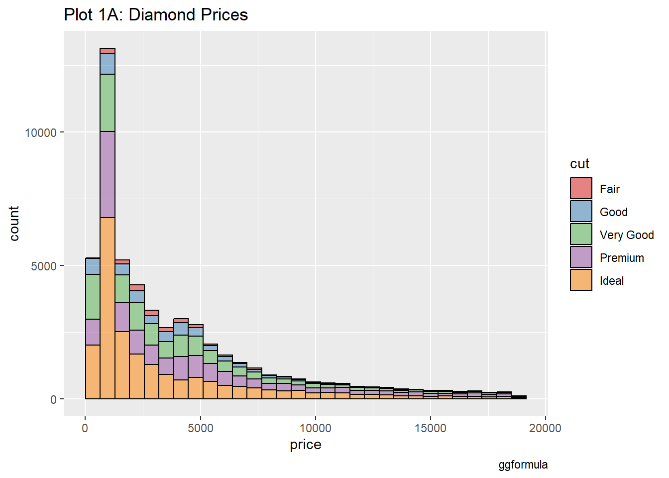
Classwork 4

Setup

library(tidyverse) # Sine qua non

── Attaching core tidyverse packages ──────────────────────── tidyverse 2.0.0 ──
✔ dplyr     1.1.4     ✔ readr     2.1.5
✔ forcats   1.0.0     ✔ stringr   1.5.1
✔ ggplot2   4.0.0     ✔ tibble    3.3.0
✔ lubridate 1.9.4     ✔ tidyr     1.3.1
✔ purrr     1.1.0     
── Conflicts ────────────────────────────────────────── tidyverse_conflicts() ──
✖ dplyr::filter() masks stats::filter()
✖ dplyr::lag()    masks stats::lag()
ℹ Use the conflicted package (<http://conflicted.r-lib.org/>) to force all conflicts to become errors

library(mosaic) # Out all-in-one package

Registered S3 method overwritten by 'mosaic':
  method                           from   
  fortify.SpatialPolygonsDataFrame ggplot2

The 'mosaic' package masks several functions from core packages in order to add 
additional features.  The original behavior of these functions should not be affected by this.

Attaching package: 'mosaic'

The following object is masked from 'package:Matrix':

    mean

The following objects are masked from 'package:dplyr':

    count, do, tally

The following object is masked from 'package:purrr':

    cross

The following object is masked from 'package:ggplot2':

    stat

The following objects are masked from 'package:stats':

    binom.test, cor, cor.test, cov, fivenum, IQR, median, prop.test,
    quantile, sd, t.test, var

The following objects are masked from 'package:base':

    max, mean, min, prod, range, sample, sum

library(ggformula) # Graphing package
library(skimr) # Looking at Data

Attaching package: 'skimr'

The following object is masked from 'package:mosaic':

    n_missing

library(janitor) # Clean the data

Attaching package: 'janitor'

The following objects are masked from 'package:stats':

    chisq.test, fisher.test

library(naniar) # Handle missing data

Attaching package: 'naniar'

The following object is masked from 'package:skimr':

    n_complete

library(visdat) # Visualise missing data
library(tinytable) # Printing Static Tables for our data

Attaching package: 'tinytable'

The following object is masked from 'package:ggplot2':

    theme_void

library(DT) # Interactive Tables for our data
library(crosstable) # Multiple variable summaries

Attaching package: 'crosstable'

The following object is masked from 'package:purrr':

    compact

Reading csv file

taxi <- read_csv("https://vincentarelbundock.github.io/Rdatasets/csv/modeldata/taxi.csv")

Rows: 10000 Columns: 8
── Column specification ────────────────────────────────────────────────────────
Delimiter: ","
chr (5): tip, company, local, dow, month
dbl (3): rownames, distance, hour

ℹ Use `spec()` to retrieve the full column specification for this data.
ℹ Specify the column types or set `show_col_types = FALSE` to quiet this message.

taxi_modified <- taxi %>%
  naniar::replace_with_na_all(condition = ~ .x %in% common_na_strings) %>%
  naniar::replace_with_na_all(condition = ~ .x %in% common_na_numbers) %>%
  janitor::clean_names(case = "snake") %>%
  janitor::remove_empty()

value for "which" not specified, defaulting to c("rows", "cols")

taxi_modified

# A tibble: 10,000 × 8
   rownames tip   distance company                      local dow   month  hour
      <dbl> <chr>    <dbl> <chr>                        <chr> <chr> <chr> <dbl>
 1        1 yes      17.2  Chicago Independents         no    Thu   Feb      16
 2        2 yes       0.88 City Service                 yes   Thu   Mar       8
 3        3 yes      18.1  other                        no    Mon   Feb      18
 4        4 yes      20.7  Chicago Independents         no    Mon   Apr       8
 5        5 yes      12.2  Chicago Independents         no    Sun   Mar      21
 6        6 yes       0.94 Sun Taxi                     yes   Sat   Apr      23
 7        7 yes      17.5  Flash Cab                    no    Fri   Mar      12
 8        8 yes      17.7  other                        no    Sun   Jan       6
 9        9 yes       1.85 Taxicab Insurance Agency Llc no    Fri   Apr      12
10       10 yes       1.47 City Service                 no    Tue   Mar      14
# ℹ 9,990 more rows

Theme chosing

RColorBrewer::display.brewer.all()

Data Munging

## Convert `dow`, `local`, `month`, and `hour` into ordered factors
taxi_modified <- taxi_modified %>%
  dplyr::mutate(

    ## Variable "tip"
    tip = base::factor(tip,
      levels = c("yes", "no"),
      labels = c("yes", "no"),
      ordered = TRUE
    ),

    ## Variable "company"
    company = base::factor(company), # Any order is OK.

    ## Variable "dow"
    dow = base::factor(dow,
      levels = c("Mon", "Tue", "Wed", "Thu", "Fri", "Sat", "Sun"),
      labels = c("Mon", "Tue", "Wed", "Thu", "Fri", "Sat", "Sun"),
      ordered = TRUE
    ),

    ## Variable "local"
    local = base::factor(local,
      levels = c("yes", "no"),
      labels = c("yes", "no"),
      ordered = TRUE
    ),

    ## Variable "month"
    month = base::factor(month,
      levels = c("Jan", "Feb", "Mar", "Apr"),
      labels = c("Jan", "Feb", "Mar", "Apr"),
      ordered = TRUE
    ),

    ## Variable "hour"
    hour = base::factor(hour,
      levels = c(0:23), labels = c(0:23),
      ordered = TRUE
    )
  ) %>%
  dplyr::relocate(where(is.factor), .after = rownames) # Move all factors to the left

taxi_modified %>% glimpse()

Rows: 10,000
Columns: 8
$ rownames <dbl> 1, 2, 3, 4, 5, 6, 7, 8, 9, 10, 11, 12, 13, 14, 15, 16, 17, 18…
$ tip      <ord> yes, yes, yes, yes, yes, yes, yes, yes, yes, yes, yes, yes, y…
$ company  <fct> Chicago Independents, City Service, other, Chicago Independen…
$ local    <ord> no, yes, no, no, no, yes, no, no, no, no, no, no, no, yes, no…
$ dow      <ord> Thu, Thu, Mon, Mon, Sun, Sat, Fri, Sun, Fri, Tue, Tue, Sun, W…
$ month    <ord> Feb, Mar, Feb, Apr, Mar, Apr, Mar, Jan, Apr, Mar, Mar, Apr, A…
$ hour     <ord> 16, 8, 18, 8, 21, 23, 12, 6, 12, 14, 18, 11, 12, 19, 17, 13, …
$ distance <dbl> 17.19, 0.88, 18.11, 20.70, 12.23, 0.94, 17.47, 17.67, 1.85, 1…

Position dodge

taxi_modified %>%
  gf_bar(~local,
    fill = ~tip,
    position = "dodge"
  ) %>%
  gf_labs(title = "Plot 2A: Dodged Bar Chart") %>%
  gf_refine(scale_fill_brewer(palette = "Set1"))

Position stack

taxi_modified %>%
  gf_bar(~local,
    fill = ~tip,
    position = "stack"
  ) %>%
  gf_labs(
    title = "Plot 2B: Stacked Bar Chart",
    subtitle = "Can we spot per group differences in proportions??"
  ) %>%
  gf_refine(scale_fill_brewer(palette = "Set1"))

Position fill

taxi_modified %>%
  gf_bar(~local,
    fill = ~tip,
    position = "fill"
  ) %>%
  gf_labs(
    title = "Plot 2C: Filled Bar Chart",
    subtitle = "Shows Per group differences in Proportions!"
  ) %>%
  gf_refine(scale_fill_brewer(palette = "Set1"))

Histogram

data("diamonds", package = "ggplot2")
glimpse(diamonds)

Rows: 53,940
Columns: 10
$ carat   <dbl> 0.23, 0.21, 0.23, 0.29, 0.31, 0.24, 0.24, 0.26, 0.22, 0.23, 0.…
$ cut     <ord> Ideal, Premium, Good, Premium, Good, Very Good, Very Good, Ver…
$ color   <ord> E, E, E, I, J, J, I, H, E, H, J, J, F, J, E, E, I, J, J, J, I,…
$ clarity <ord> SI2, SI1, VS1, VS2, SI2, VVS2, VVS1, SI1, VS2, VS1, SI1, VS1, …
$ depth   <dbl> 61.5, 59.8, 56.9, 62.4, 63.3, 62.8, 62.3, 61.9, 65.1, 59.4, 64…
$ table   <dbl> 55, 61, 65, 58, 58, 57, 57, 55, 61, 61, 55, 56, 61, 54, 62, 58…
$ price   <int> 326, 326, 327, 334, 335, 336, 336, 337, 337, 338, 339, 340, 34…
$ x       <dbl> 3.95, 3.89, 4.05, 4.20, 4.34, 3.94, 3.95, 4.07, 3.87, 4.00, 4.…
$ y       <dbl> 3.98, 3.84, 4.07, 4.23, 4.35, 3.96, 3.98, 4.11, 3.78, 4.05, 4.…
$ z       <dbl> 2.43, 2.31, 2.31, 2.63, 2.75, 2.48, 2.47, 2.53, 2.49, 2.39, 2.…

diamonds_modified <- diamonds %>%
  janitor::clean_names(case = "snake") %>%
  janitor::remove_empty(which = c("rows", "cols")) # Empty columns and rows if any
diamonds_modified %>% glimpse()

Rows: 53,940
Columns: 10
$ carat   <dbl> 0.23, 0.21, 0.23, 0.29, 0.31, 0.24, 0.24, 0.26, 0.22, 0.23, 0.…
$ cut     <ord> Ideal, Premium, Good, Premium, Good, Very Good, Very Good, Ver…
$ color   <ord> E, E, E, I, J, J, I, H, E, H, J, J, F, J, E, E, I, J, J, J, I,…
$ clarity <ord> SI2, SI1, VS1, VS2, SI2, VVS2, VVS1, SI1, VS2, VS1, SI1, VS1, …
$ depth   <dbl> 61.5, 59.8, 56.9, 62.4, 63.3, 62.8, 62.3, 61.9, 65.1, 59.4, 64…
$ table   <dbl> 55, 61, 65, 58, 58, 57, 57, 55, 61, 61, 55, 56, 61, 54, 62, 58…
$ price   <int> 326, 326, 327, 334, 335, 336, 336, 337, 337, 338, 339, 340, 34…
$ x       <dbl> 3.95, 3.89, 4.05, 4.20, 4.34, 3.94, 3.95, 4.07, 3.87, 4.00, 4.…
$ y       <dbl> 3.98, 3.84, 4.07, 4.23, 4.35, 3.96, 3.98, 4.11, 3.78, 4.05, 4.…
$ z       <dbl> 2.43, 2.31, 2.31, 2.63, 2.75, 2.48, 2.47, 2.53, 2.49, 2.39, 2.…

gf_histogram(~price, data = diamonds_modified, fill=~cut, color="black") %>%
  gf_labs(
    title = "Plot 1A: Diamond Prices",
    caption = "ggformula"
  ) %>% 
  gf_refine(scale_fill_brewer(palette = "Set1"))

`stat_bin()` using `bins = 30`. Pick better value `binwidth`.

gf_histogram(~price | cut, data = diamonds_modified, fill=~cut, color="black") %>%
  gf_labs(
    title = "Plot 1A: Diamond Prices",
    caption = "ggformula"
  ) %>% 
  gf_refine(scale_fill_brewer(palette = "Set8"))

Warning: Unknown palette: "Set8"

`stat_bin()` using `bins = 30`. Pick better value `binwidth`.

gf_histogram(~price | color, data = diamonds_modified, fill=~color, color="black") %>%
  gf_labs(
    title = "Plot 1A: Diamond Prices",
    caption = "ggformula"
  ) %>% 
  gf_refine(scale_fill_brewer(palette = "Set1"))

`stat_bin()` using `bins = 30`. Pick better value `binwidth`.

glimpse(diamonds_modified)

Rows: 53,940
Columns: 10
$ carat   <dbl> 0.23, 0.21, 0.23, 0.29, 0.31, 0.24, 0.24, 0.26, 0.22, 0.23, 0.…
$ cut     <ord> Ideal, Premium, Good, Premium, Good, Very Good, Very Good, Ver…
$ color   <ord> E, E, E, I, J, J, I, H, E, H, J, J, F, J, E, E, I, J, J, J, I,…
$ clarity <ord> SI2, SI1, VS1, VS2, SI2, VVS2, VVS1, SI1, VS2, VS1, SI1, VS1, …
$ depth   <dbl> 61.5, 59.8, 56.9, 62.4, 63.3, 62.8, 62.3, 61.9, 65.1, 59.4, 64…
$ table   <dbl> 55, 61, 65, 58, 58, 57, 57, 55, 61, 61, 55, 56, 61, 54, 62, 58…
$ price   <int> 326, 326, 327, 334, 335, 336, 336, 337, 337, 338, 339, 340, 34…
$ x       <dbl> 3.95, 3.89, 4.05, 4.20, 4.34, 3.94, 3.95, 4.07, 3.87, 4.00, 4.…
$ y       <dbl> 3.98, 3.84, 4.07, 4.23, 4.35, 3.96, 3.98, 4.11, 3.78, 4.05, 4.…
$ z       <dbl> 2.43, 2.31, 2.31, 2.63, 2.75, 2.48, 2.47, 2.53, 2.49, 2.39, 2.…

diamonds_modified %>%
  gf_boxplot(cut ~ carat | clarity, orientation = "y") %>%
  gf_labs(y = "Gender", x = "Income", title = "Plot 2A: Income by Gender")

diamonds_modified %>%
  gf_boxplot(clarity ~ depth, orientation = "y") %>%
  gf_labs(y = "Gender", x = "Income", title = "Plot 2A: Income by Gender")

diamonds_modified %>%
  gf_boxplot(color ~ price, orientation = "y", fill = "pink", color = "black") %>%
  gf_labs(y = "Gender", x = "Income", title = "Plot 2A: Income by Gender")

diamonds_modified %>%
  gf_boxplot(clarity ~ price, orientation = "y") %>%
  gf_labs(y = "Clarity", x = "Price", title = "Plot 2A: Income by Gender")

diamonds_modified %>%
  gf_boxplot(cut ~ carat, orientation = "y") %>%
  gf_labs(y = "Clarity", x = "Price", title = "Plot 2A: Income by Gender")